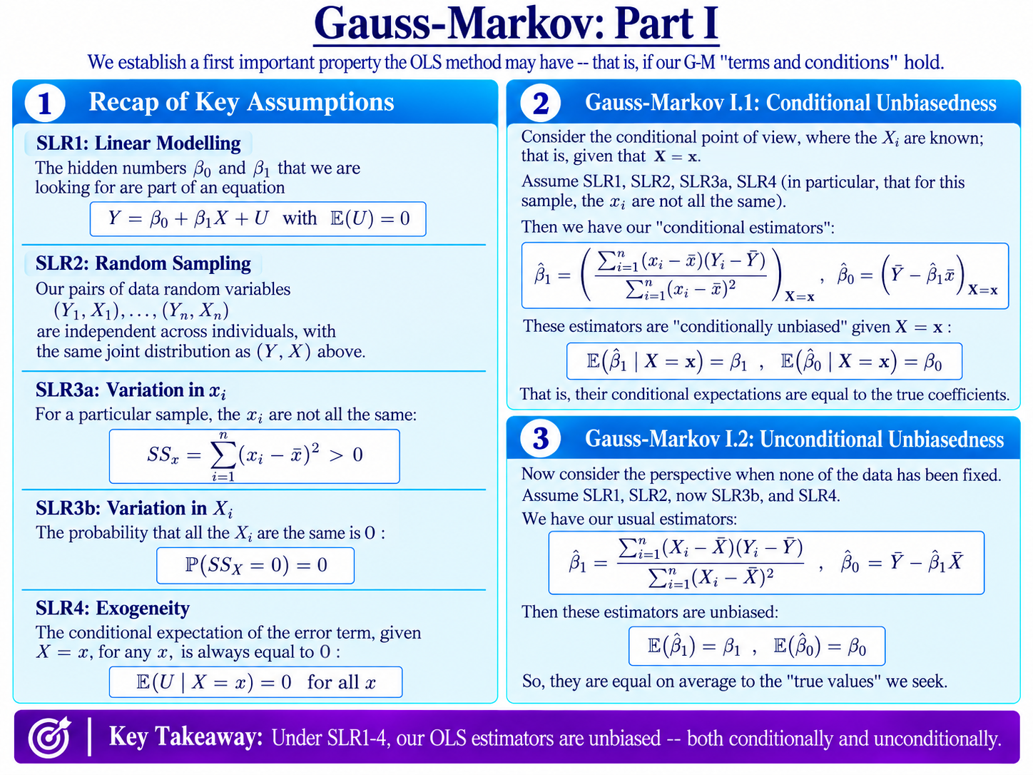
Gauss-Markov: Part I

We have now carefully introduced our first four assumptions for simple linear regression.

It’s time to see what we get in return!

We can now prove the first part of the Gauss-Markov theorem, concerning unbiasedness.

There are actually two versions of the first-part result, corresponding to the two points of view we have already introduced.

First, conditional on the observed values of $X$, OLS is conditionally unbiased. Then, under a slightly stronger variation assumption, we can remove this conditioning and establish ordinary or unconditional unbiasedness.

We will also pay careful attention to which assumptions do what in the proof.

Theorem 1: Conditional Unbiasedness

Consider first the conditional point of view. Write

$$\mathbf{X}=(X_1,\ldots,X_n)$$

and suppose we have observed

$$\mathbf{X}=\mathbf{x}=(x_1,\ldots,x_n).$$

The $x_i$ are now fixed numbers, while the $Y_i$ – and therefore our OLS estimators – remain random variables.

We might write them as follows:

$$\hat\beta_1\big|_{\mathbf{X}=\mathbf{x}}$$

and

$$\hat\beta_0\big|_{\mathbf{X}=\mathbf{x}}$$

Now, suppose that SLR1, SLR2, SLR3a and SLR4 hold.

Then

$$\mathbb{E}(\hat\beta_1\mid\mathbf{X}=\mathbf{x})=\beta_1$$

and

$$\mathbb{E}(\hat\beta_0\mid\mathbf{X}=\mathbf{x})=\beta_0.$$

That is, conditional on any set of observed $x_i$ satisfying SLR3a, our OLS estimators are centred on the particular coefficients $\beta_0$ and $\beta_1$ we are seeking.

Theorem 2: Unconditional Unbiasedness

We can also return to the point of view before any of the $X_i$ have been observed.

Now suppose that SLR1, SLR2, SLR3b and SLR4 hold.

Then

$$\mathbb{E}(\hat\beta_1)=\beta_1$$

and

$$\mathbb{E}(\hat\beta_0)=\beta_0.$$

So, over different random samples, our OLS estimators are centred on the coefficients $\beta_0$ and $\beta_1$ we are seeking.

The change from the conditional result is that we switch to the unconditional point of view, and SLR3a is replaced by SLR3b.

Assumptions for the Two Results

Before giving the proof, we recap the assumptions needed for easy reference.

SLR1: Linear Modelling

$$Y=\beta_0+\beta_1X+U,\qquad \mathbb{E}(U)=0.$$

SLR2: Random Sampling

$$(Y_1,X_1,U_1),\ldots,(Y_n,X_n,U_n)\ \text{are i.i.d. copies of }(Y,X,U).$$

SLR3a: Variation in the Observed $x_i$

$$SS_x=\sum_{i=1}^{n}(x_i-\bar{x})^2>0.$$

SLR3b: Variation Before Sampling

$$\mathbb{P}(SS_X=0)=0,\qquad SS_X=\sum_{i=1}^{n}(X_i-\bar{X})^2.$$

SLR4: Exogeneity

$$\mathbb{E}(U\mid X=x)=0\qquad \text{for all }x.$$

For conditional unbiasedness we use SLR1, SLR2, SLR3a and SLR4.

For unconditional unbiasedness we use SLR1, SLR2, SLR3b and SLR4.

Proof 1: Conditional Unbiasedness

Let’s prove the result for the slope first.

Under SLR3a,

$$SS_x=\sum_{i=1}^{n}(x_i-\bar{x})^2>0,$$

so the OLS slope estimator based on the usual formula is well-defined.

We begin with its conditional expectation:

$$\mathbb{E}(\hat\beta_1\mid\mathbf{X}=\mathbf{x})=\mathbb{E}\left(\frac{\sum_{i=1}^{n}(x_i-\bar{x})(Y_i-\bar{Y})}{\sum_{i=1}^{n}(x_i-\bar{x})^2}\mid\mathbf{X}=\mathbf{x}\right)$$

Since $\sum_{i=1}^{n}(x_i-\bar{x})=0$, the term involving $\bar{Y}$ disappears:

$$=\mathbb{E}\left(\frac{\sum_{i=1}^{n}(x_i-\bar{x})Y_i}{\sum_{i=1}^{n}(x_i-\bar{x})^2}\mid\mathbf{X}=\mathbf{x}\right)$$

Conditional on $\mathbf{X}=\mathbf{x}$, all the $x_i$ are fixed numbers, so we can take them outside the expectation:

$$=\frac{\sum_{i=1}^{n}(x_i-\bar{x})\mathbb{E}(Y_i\mid\mathbf{X}=\mathbf{x})}{\sum_{i=1}^{n}(x_i-\bar{x})^2}$$

By SLR1 and SLR2 together, we can replace $Y_i$ with its population line formula, $\beta_0+\beta_1X_i+U_i$:

$$=\frac{\sum_{i=1}^{n}(x_i-\bar{x})\left(\mathbb{E}(\beta_0+\beta_1X_i+U_i\mid\mathbf{X}=\mathbf{x})\right)}{\sum_{i=1}^{n}(x_i-\bar{x})^2}$$

Again, we move known terms outside the brackets:

$$=\frac{\sum_{i=1}^{n}(x_i-\bar{x})\left(\beta_0+\beta_1x_i+\mathbb{E}(U_i\mid\mathbf{X}=\mathbf{x})\right)}{\sum_{i=1}^{n}(x_i-\bar{x})^2}$$

As above, since $\sum_{i=1}^{n}(x_i-\bar{x})=0$, the term involving $\beta_0$ disappears. Also, because of SLR2 again, $U_i$ is independent of all $X_j$ for $j≠i$. Hence, conditioning on the rest of the sample does not matter:

$$=\frac{\sum_{i=1}^{n}(x_i-\bar{x})\left(\beta_1x_i+\mathbb{E}(U_i \mid X_i=x_i)\right)}{\sum_{i=1}^{n}(x_i-\bar{x})^2}$$

We now use SLR2 and SLR4 together. By SLR2, each $(X_i,U_i)$ is a copy of $(X,U)$, so SLR4 gives $\mathbb{E}(U_i\mid X_i=x_i)=0.$ We then obtain:

$$=\frac{\sum_{i=1}^{n}(x_i-\bar{x})\left(\beta_1x_i+0\right)}{\sum_{i=1}^{n}(x_i-\bar{x})^2}=\frac{\beta_1 \sum_{i=1}^{n}(x_i-\bar{x})x_i}{\sum_{i=1}^{n}(x_i-\bar{x})^2}$$

Finally, again using $\sum_{i=1}^{n}(x_i-\bar{x})=0$, we can subtract the fixed term $\bar{x}$ from the second factor:

$$=\beta_1\frac{ \sum_{i=1}^{n}(x_i-\bar{x})(x_i-\bar{x})}{\sum_{i=1}^{n}(x_i-\bar{x})^2}=\beta_1$$

Hence, we have shown:

$$\mathbb{E}(\hat\beta_1\mid\mathbf{X}=\mathbf{x})=\beta_1.$$

So, the OLS slope estimator is conditionally unbiased. Phew!

Now, for the intercept, recall that

$$\hat\beta_0=\bar{Y}-\hat\beta_1\bar{X}.$$

Taking the conditional expectation,

$$\mathbb{E}(\hat\beta_0\mid\mathbf{X}=\mathbf{x})=\mathbb{E}(\bar{Y}\mid\mathbf{X}=\mathbf{x})-\bar{x}\mathbb{E}(\hat\beta_1\mid\mathbf{X}=\mathbf{x}).$$

From SLR1, SLR2 and SLR4, we have that $\mathbb{E}(Y_i\mid\mathbf{X}=\mathbf{x})=\beta_0+\beta_1x_i,$ for each $i$. So, averaging these, $\mathbb{E}(\bar{Y}\mid\mathbf{X}=\mathbf{x})=\beta_0+\beta_1\bar{x}.$ So, substituting this in, we get:

$$=\beta_0+\beta_1\bar{x}-\bar{x}\mathbb{E}(\hat\beta_1\mid\mathbf{X}=\mathbf{x})$$

Using the slope result just proved for the final term,

$$=\beta_0+\beta_1\bar{x}-\bar{x}\beta_1 = \beta_0$$

and therefore

$$\mathbb{E}(\hat\beta_0\mid\mathbf{X}=\mathbf{x})=\beta_0.$$

Thus both OLS estimators are conditionally unbiased.

Proof 2: Unconditional Unbiasedness

We now prove the second result.

Here the $X_i$ are random again, so we use SLR3b rather than SLR3a:

$$\mathbb{P}(SS_X=0)=0.$$

We may define $\hat\beta_1$ to take any convenient value when $SS_X=0$, such as $0$. Since this event has probability $0$, that choice cannot affect its expectation.

We can now apply our usual three-step method for the Law of Iterated Expectation.

Step 1: Condition on $\mathbf{X}=\mathbf{x}$

From the first theorem,

$$\mathbb{E}(\hat\beta_1\mid\mathbf{X}=\mathbf{x})=\beta_1$$

whenever $SS_x>0$.

This is exactly the conditional result proved above. But under SLR3b,

$$\mathbb{P}(SS_X>0)=1.$$

So this conditional equality holds with probability 1.

Step 2: Bring $\mathbf{x}$ Back to Life

Our next step is to replace the fixed vector $\mathbf{x}$ with the random vector $\mathbf{X}$.

Thus

$$\mathbb{E}(\hat\beta_1\mid\mathbf{X})=\beta_1$$

with probability 1.

Notice that nothing actually changes on the right-hand side when we bring $\mathbf{x}$ back to life. $\beta_1$ is a fixed constant – it never depended on the particular values $\mathbf{x}$ in the first place!

Step 3: Take an Expectation Again

Finally, the Law of Iterated Expectation gives

$$\mathbb{E}(\hat\beta_1)=\mathbb{E}\left(\mathbb{E}(\hat\beta_1\mid\mathbf{X})\right).$$

So, using the result from Step 2,

$$\mathbb{E}(\hat\beta_1)=\mathbb{E}(\beta_1)=\beta_1.$$

That is, the OLS slope estimator is unconditionally unbiased.

The Unconditional Intercept

The same three steps apply to the intercept.

From our first theorem,

$$\mathbb{E}(\hat\beta_0\mid\mathbf{X}=\mathbf{x})=\beta_0$$

whenever $SS_x>0$.

By SLR3b, this holds with probability 1. Bringing $\mathbf{x}$ back to life therefore gives

$$\mathbb{E}(\hat\beta_0\mid\mathbf{X})=\beta_0$$

with probability 1.

Finally, applying the Law of Iterated Expectation,

$$\mathbb{E}(\hat\beta_0)=\mathbb{E}\left(\mathbb{E}(\hat\beta_0\mid\mathbf{X})\right)=\mathbb{E}(\beta_0)=\beta_0.$$

Thus both OLS estimators are unconditionally unbiased!

Background

• Conditional Expectations
• Law of Iterated Expectation
• Applying the Law of Iterated Expectation
• Estimators as Random Variables
• Unbiasedness
• Conditioning on X
• SLR1: Linear Modelling
• SLR2: Random Sampling
• SLR3: Variation in X
• SLR4: Exogeneity