The Homoskedasticity Assumption

We have so far focused mainly on the expected value of the error term.

SLR5 turns instead to its variance.

Consider our usual linear model:

$$Y=\beta_0+\beta_1X+U.$$

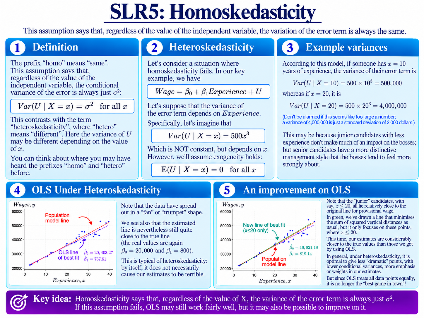
The prefix “homo” means “same”. The homoskedasticity assumption says that, regardless of the value of the independent variable, the conditional variance of the error term $U$ is always the same:

$$\operatorname{Var}(U\mid X=x)=\sigma^2\qquad\text{for all }x.$$

Here, $\sigma^2$ is some fixed but unknown number.

So, learning that $X=x$ may tell us which part of the population we are looking at, but it should not tell us that the error term is likely to be more or less widely spread out.

This is quite different from SLR4: Exogeneity, which concerned the conditional expectation:

$$\mathbb{E}(U\mid X=x)=0.$$

SLR4 asks whether the error tends to point upwards or downwards at different values of $X$.

SLR5 asks whether the size of its variation changes.

Homoskedasticity and Heteroskedasticity

When

$$\operatorname{Var}(U\mid X=x)=\sigma^2$$

for every $x$, we say that the errors are homoskedastic.

If instead the conditional variance changes with $x$, we say that the errors are heteroskedastic. Sometimes the spellings homoscedastic and heteroscedastic are used.

For example, suppose

$$\operatorname{Var}(U\mid X=x)=500x^3.$$

This is clearly not constant. Larger values of $X$ are associated with a larger conditional variance of the error term.

So, this population model exhibits heteroskedasticity.

Notice that this says nothing by itself about exogeneity. We could perfectly well have both

$$\mathbb{E}(U\mid X=x)=0$$

and

$$\operatorname{Var}(U\mid X=x)=500x^3.$$

The errors would still balance out around $0$ on average at every value of $X$ – but their spread around $0$ would become larger as $X$ increases.

Our Wage Example

Return to the model

$$Wage=\beta_0+\beta_1Experience+U.$$

Suppose $U$ again represents the adjustment to someone’s wage produced by how the bosses react to them.

It is quite plausible that this adjustment might be relatively modest for junior workers, while becoming much more variable for senior workers.

Perhaps junior candidates are still fairly similar from the bosses’ point of view. Senior candidates, on the other hand, may have developed more distinctive personalities or management styles, which the bosses may either like very much or dislike quite strongly.

The average adjustment could still be $0$ at every level of experience.

But the variance of that adjustment could increase with experience.

For our numerical example,

$$\operatorname{Var}(U\mid X=x)=500x^3.$$

At $x=10$,

$$\operatorname{Var}(U\mid X=10)=500\times10^3=500{,}000.$$

At $x=20$,

$$\operatorname{Var}(U\mid X=20)=500\times20^3=4{,}000{,}000.$$

So, the errors are simply much more widely dispersed for workers with more experience.

If you are worried that these variances look enormous, remember that variance is measured in squared units. A variance of $4{,}000{,}000$ dollars squared corresponds to a standard deviation of only

$$\sqrt{4{,}000{,}000}=$2{,}000.$$

What Does Heteroskedasticity Look Like?

The graph on the slide shows the consequences of heteroskedasticity.

At low levels of experience, the observations sit relatively close to the population line.

As experience increases, they spread further above and below it.

The shape that emerges is often described as a fan, though here it looks more like a trumpet.

Notice that for each value of $x$ the points are still about equally pushed off up or down from the population line, and indeed, this particular dataset was based on a model that also satisfies exogeneity:

$$\mathbb{E}(U\mid X=x)=0.$$

It is only the spread around the population line that changes with $x$: that is, the conditional distribution of $U$ is narrow for some values of $x$ and wide for others.

Does Heteroskedasticity Ruin the OLS Method?

If we have heteroskedasticity, does everything go wrong? Not necessarily!

This is an important contrast with exogeneity.

In Gauss-Markov – Part I, we proved that OLS is unbiased using SLR1–SLR4.

We did not use SLR5.

So if homoskedasticity fails while the earlier assumptions continue to hold, OLS will still be unbiased – both conditionally and unconditionally. Heteroskedasticity by itself therefore does not make OLS biased.

So, in any one sample, the OLS line may still lie quite close to the population line, as it does on the slide.

However, whilst it is still unbiased, the situation becomes less than ideal for OLS. One reason for this is given below; other reasons will be discussed in more advanced topics.

Can We Do Better Than OLS?

The final graph on the slide gives us a clue about one reason why homoskedasticity will nevertheless matter.

Some observations are much more tightly concentrated around the population line than others.

The junior workers have relatively low conditional error variances, while the senior workers are much more widely dispersed.

Ordinary least squares treats every squared residual equally.

But if we know that some observations are much less variable than others, it seems plausible that we might want to place more weight on the more precise observations and less weight on the noisier ones.

The green line on the slide illustrates the idea by fitting the line of best fit using only the lower-variance junior observations. In this particular sample, it happens to land considerably closer to the true population line than ordinary OLS.

Throwing away the noisier observations is not generally the best method. A more sophisticated approach would still use all the data, while placing greater weight on observations with lower conditional variance.

The important point for now is simply this:

When the error variance changes with $X$, OLS may remain unbiased, but other methods may make better use of the information in our data.

This is exactly where SLR5 will enter the next part of the Gauss-Markov theorem. If SLR5 does hold, along with our other assumptions, then this cannot happen – OLS is, in a particular sense, the best method of its sort that we could use.

A Useful Warning

Homoskedasticity is sometimes carelessly written as

$$\operatorname{Var}(U_i)=\sigma^2\qquad\text{for every }i.$$

That is not the assumption we need.

Under SLR2: Random Sampling, the $U_i$ already have the same unconditional distribution as one another. So, assuming the variance exists,

$$\operatorname{Var}(U_i)=\operatorname{Var}(U)$$

for every $i$ anyway.

Thus, merely saying that all the $U_i$ have the same unconditional variance does not give us SLR5.

Homoskedasticity says something stronger and different:

$$\operatorname{Var}(U\mid X=x)=\sigma^2\qquad\text{for every }x.$$

It is the conditional variance that must remain constant as $x$ changes.

Combining SLR2 with SLR5 then gives, for each member of our random sample,

$$\operatorname{Var}(U_i\mid X_i=x_i)=\sigma^2.$$

And, from the conditional point of view used in our Gauss-Markov proofs,

$$\operatorname{Var}(U_i\mid\mathbf{X}=\mathbf{x})=\sigma^2.$$

So every observation has the same conditional error variance once the $x$-data have been fixed.

Background

• Variance and Standard Deviation
• Conditional Expectations
• Conditional Variance and the Law of Total Variance
• Unbiasedness
• Conditioning on X
• SLR2: Random Sampling
• SLR4: Exogeneity
• Gauss-Markov – Part I