The First SLR Assumption

We now introduce the first of our assumptions for simple linear regression.

SLR1: Linear Modelling says that the population variables $Y$, $X$ and $U$ are related by the unknown numbers $\beta_0$ and $\beta_1$ in the usual linear model formula:

$$Y=\beta_0+\beta_1X+U,$$

where the expected value of the error term is $0$:

$$\mathbb{E}(U)=0.$$

This seems simple enough – but actually it raises a lot of tricky questions!

Below, we will navigate these thorny issues in a flexible way that avoids committing to answering them head-on. But before this, we first present the practical importance of the assumption.

Why Do We Need $\mathbb{E}(U)=0$?

In our wages example, the condition

$$\mathbb{E}(U)=0$$

says that the error term may push individual wages above or below the linear part of the model, but does not push them systematically in one direction overall.

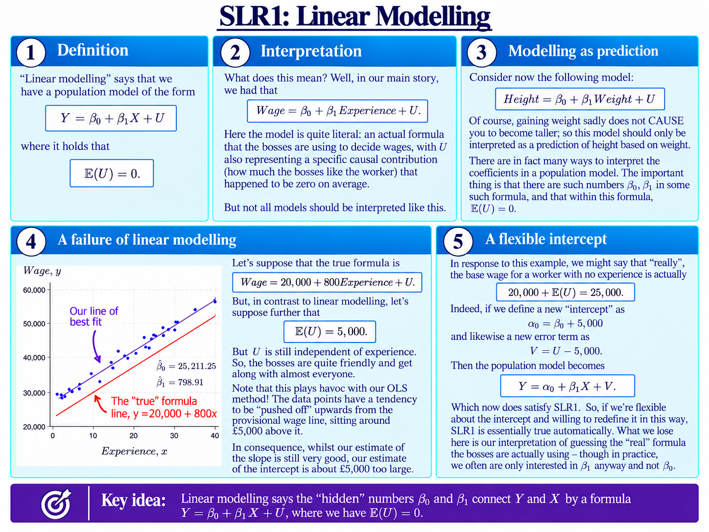
The slide shows what happens if instead

$$\mathbb{E}(U)=5{,}000.$$

The observations now tend to sit around £5,000 above the original model line. So, an OLS line fitted through those observations will naturally tend to sit above it too.

The graph makes the problem quite obvious: if the data are simply not centred around the line whose coefficients we are trying to estimate, a line that matches them won’t match the line either.

In the particular example shown on the slide, our estimate of the original intercept $\beta_0$ consequently tends to be around £5,000 too high.

Next, we move on to a more detailed discussion of the meaning of SLR1. This part of the page will be rather more philosophical than most; read on if you dare!

What SLR1 Does Not Mean

One possible interpretation is that SLR1 simply says there exist some numbers $\beta_0$ and $\beta_1$, and some corresponding error term $U$, for which

$$Y=\beta_0+\beta_1X+U$$

and

$$\mathbb{E}(U)=0.$$

But interpreted like this, the assumption is entirely trivial, and not of interest!

For example, suppose we choose

$$\beta_0=\mathbb{E}(Y)$$

and

$$\beta_1=0.$$

Now define

$$U=Y-\mathbb{E}(Y).$$

Then automatically

$$Y=\beta_0+\beta_1X+U,$$

and

$$\mathbb{E}(U)=0.$$

Yet we have assumed nothing whatsoever about $X$, and almost nothing about $Y$ beyond the existence of its expected value!

So, SLR1 would be fairly pointless if it simply meant this. We should consider another possibility instead.

A Stronger Interpretation

We could instead start by thinking of $Y$, $X$ and $U$ as three separately meaningful population random variables, connected by a formula:

$$Y=\beta_0+\beta_1X+U.$$

This is how we have often imagined our wages example:

$$Wage=\beta_0+\beta_1Experience+U,$$

where $U$ specifically represents the bosses’ adjustment to wages based on how much they like them in an initial meeting.

When interpreted like this, we call the equation a structural model.

On this interpretation, the equation is certainly not trivial. Indeed, the bosses might instead have used some quite different rule, such as

$$Y=\alpha_0+\alpha_1\sqrt{X}+U.$$

Now, many researchers do indeed think of their models like this, and the structural view can be useful and valid. However, it is quite restrictive as a general interpretation of linear regression.

In particular, there are many other applications of OLS where we do not want to think of $U$ as some independently existing causal factor. For instance, it may instead simply be whatever is left over in determining $Y$ after accounting for the effect of $X$; and, unlike our stylised example, this may consist of many disparate things lumped together.

In the next section, then, we advocate a more neutral approach.

The Quest for the Coefficients: User-Friendly Gauss-Markov

On this view, we will take as primary the fact that there are some particular unknown numbers $\beta_0$ and $\beta_1$ that we care about and would like OLS to estimate. But we also allow precisely what these numbers mean to depend on the application.

As above, they might, for example, reflect a genuine causal relationship we want to learn about; or alternatively, just be numbers that provide a useful linear prediction of $Y$ based on $X$.

Whatever the interpretation, once the coefficients we care about have been specified, we define the corresponding error term as

$$U=Y-\beta_0-\beta_1X.$$

SLR1 then requires that, for these numbers we are looking for in the present application, however we understand them, the resulting error term should satisfy

$$\mathbb{E}(U)=0.$$

Recentering the Error Term

We return to the problem shown on the slide; a situation where $\mathbb{E}(U)\ne0$.

In situations like this, there is a mathematical manoeuvre available to remedy the situation.

Starting from

$$Y=\beta_0+\beta_1X+U,$$

we can rewrite the same model as

$$Y=(\beta_0+\mathbb{E}(U))+\beta_1X+(U-\mathbb{E}(U)).$$

Now define a new intercept

$$\alpha_0=\beta_0+\mathbb{E}(U)$$

and a new error term

$$V=U-\mathbb{E}(U).$$

Then

$$Y=\alpha_0+\beta_1X+V,$$

where

$$\mathbb{E}(V)=0.$$

So we can always recentre the error term by absorbing its average value into the intercept.

But notice what has happened: we have changed the intercept we are trying to estimate.

Does This Matter?

Whether we will be satisfied by this move depends on what our goals are in the application at hand; in particular, on what $\beta_0$ means to us.

If $\beta_0$ had some substantive interpretation of its own – for example, if it literally was the constant used by the bosses in their wage formula – then replacing it with $\alpha_0$ means giving up on estimating that original constant.

In that setting, $\mathbb{E}(U)=0$ really is a substantive assumption.

If, on the other hand, we take a flexible attitude to the constant, perhaps as just being whatever it needs to be to make a good prediction of $Y$ based on $X$, then allowing it to be redefined as above causes us much less difficulty.

Things are admittedly easier if we are willing to let the assumptions influence how our coefficients are defined, rather than thinking of them as having a fixed pre-existing meaning and then hoping the assumptions happen to hold. Depending on our purposes, though, this may not be what we want!

Fortunately, for SLR1 at least, in many econometric applications the intercept is not our main object of interest anyway. We are usually much more interested in the slope $\beta_1.$ And the recentering above changes the intercept while leaving that slope untouched.

Summary: What SLR1 Does

We have raised some interesting interpretive questions, but noted that on the present theoretical approach we can leave these questions open.

As we will understand it here, SLR1 – like the other Gauss-Markov assumptions – does not itself supply an interpretation of the coefficients. Rather, its contribution is towards answering the question of whether OLS can reliably recover the particular coefficients $\beta_0$ and $\beta_1$ that we are interested in finding.

So, we allow for individual econometricians using the theorem to give their own interpretation of the coefficients and resulting model. What we insist on with SLR1 is that once this is done, and once we thus define

$$U=Y-\beta_0-\beta_1X,$$

we end up with

$$\mathbb{E}(U)=0.$$

In particular, any additional assumptions about how $U$ itself should be understood – whether as a real factor, or just a statistical leftover – are seen as optional, and left to the particular application.

As long as our two equations hold for the numbers $\beta_0$ and $\beta_1$ we are seeking – so far, so good!

Background

• Expected Values
• Linear Models
• Evaluating OLS: Gauss-Markov