The Exogeneity Assumption

We now come to perhaps the most important of the Gauss-Markov assumptions.

SLR4: Exogeneity says that, for every possible value $x$ of the independent variable, the conditional expectation of the error term is $0$:

$$\mathbb{E}(U\mid X=x)=0.$$

We already assumed in SLR1 that

$$\mathbb{E}(U)=0.$$

Exogeneity says something stronger: even after we learn that $X=x$, the expected value of the error term must still remain $0$.

So, knowing the value of $X$ should not tell us whether the error term is likely to push $Y$ upwards or downwards on average.

Exogeneity and the Population Line

Starting from our linear model

$$Y=\beta_0+\beta_1X+U,$$

we can condition on $X=x$:

$$\mathbb{E}(Y\mid X=x)=\beta_0+\beta_1x+\mathbb{E}(U\mid X=x).$$

Under exogeneity,

$$\mathbb{E}(U\mid X=x)=0,$$

and hence

$$\mathbb{E}(Y\mid X=x)=\beta_0+\beta_1x.$$

So, when SLR4 holds, our population line gives the conditional expectation of $Y$ for each given value $X=x$.

What Happens When Exogeneity Fails?

Return to our main example:

$$Wage=\beta_0+\beta_1Experience+U.$$

Here, $U$ represents how much the bosses happen to like a worker when they meet them.

Suppose now that the bosses tend to get on better with older workers, since they are a little older themselves. Since workers with more experience also tend to be older, workers with higher experience may now tend to have larger error terms.

For a simple mathematical example, suppose

$$\mathbb{E}(U\mid X=x)=200x-4{,}000.$$

A worker with $40$ years of experience then has expected error

$$200\times40-4{,}000=4{,}000,$$

whereas a worker with no experience has expected error

$$200\times0-4{,}000=-4{,}000.$$

So the error is systematically pushing wages downwards at low values of experience and upwards at high values.

What This Does to OLS

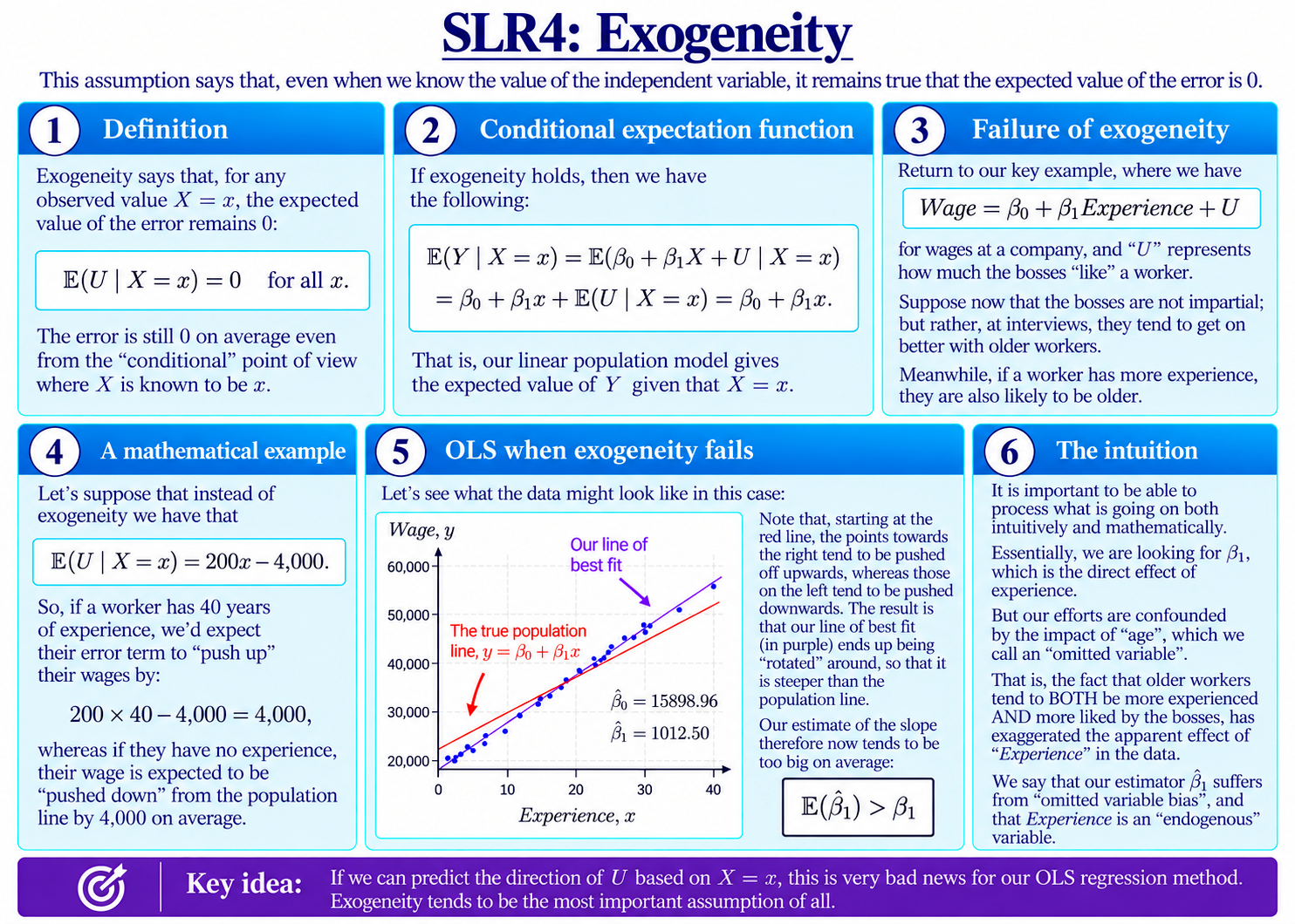
The graph on the slide shows the consequence.

The true population line is still at $y=20{,}000+800x$ as before. But now, as expected, observations towards the left tend to be pushed downwards, while those towards the right tend to be pushed upwards.

As a result, the line of best fit appears to be rotated and is much steeper than the population line.

So, our estimate of the slope is too large:

$$\hat\beta_1>\beta_1$$ $$1012.50>800$$

Our estimate of the intercept is quite off target too!

The Intuition: Distorting the Effect

Intuitively, the facts that more experienced workers tend to be older, and that the bosses happen to like older workers too, together have the effect of exaggerating the apparent causal effect of experience in the data.

As $X$ increases, there is a direct effect we are trying to measure, as represented by $\beta_1$ in the official formula for wages. However, there is also a further, indirect effect on what we’d expect $Y$ to be at these higher levels of $X$. That is, more experienced workers are likely to be older, and this tends to push up the error term too.

The two effects become mixed together in the data, and OLS ends up measuring the total predicted change in $Y$ as $X$ moves – which is not what we want.

In particular, the conditional expectation is now not the same as our original linear model. For the specific values $\beta_0=20{,}000$ and $\beta_1=800$,

$$\mathbb{E}(Y\mid X=x)=20{,}000+800x+\mathbb{E}(U\mid X=x)$$

and hence

$$\mathbb{E}(Y\mid X=x)=20{,}000+800x+200x-4{,}000=16{,}000+1{,}000x.$$

Notice that our OLS estimates of the slope and intercept actually are very close to those of this conditional expectation function – the line the data actually sit close to.

So, if we had only been trying to predict wages based on experience, rather than recover the causal effect in the original formula, this particular problem would disappear.

This is comforting! However, we may of course be specifically interested in the causal effect: for instance, the value of gaining another year of experience ourselves before joining – assuming we won’t become more or less likeable to the bosses in the meantime, as the age gap has not narrowed. So, whether OLS “works well” also depends on what we use it for!

Finally, in other cases there may be no straight line that the data sit near at all; they might follow some quite different pattern, such as a curve.

Endogeneity

In general, when exogeneity fails, we say that $X$ is endogenous.

In our example, age is an omitted variable: it affects wages through the error term, while also being related to experience. The resulting distortion is an example of omitted variable bias.

We will study endogeneity and omitted variables in much more detail later on. For now, the key idea is simply this:

If knowing $X=x$ helps us predict the direction of the error, OLS is going to have a bad time!

This is exactly what SLR4 rules out.

Background

• Conditional Expectations
• Evaluating OLS: Gauss-Markov
• Conditioning on X
• SLR1: Linear Modelling