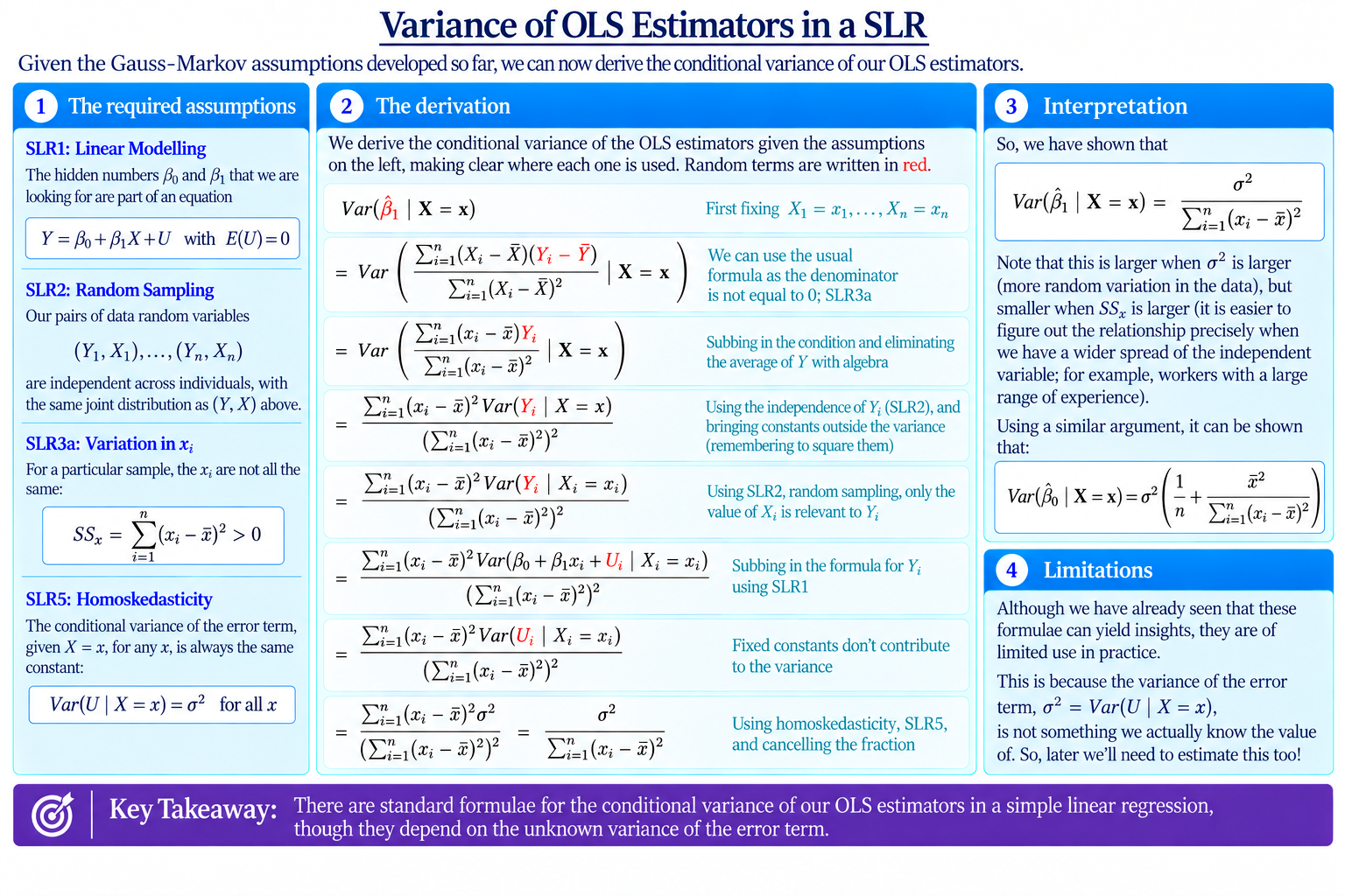
Conditional Variance of the OLS Estimators

So far, we have focused on the expected values of our OLS estimators.

Under SLR1–SLR4, we found that OLS is unbiased.

We now turn to another important feature of these estimators: their variance.

Trying to find the unconditional variance of OLS is rather difficult, because the $X_i$ are themselves random and occur in the formula in complicated ways.

So, for this topic, we return to our conditional point of view.

That is, we fix

$$\mathbf{X}=\mathbf{x}=(x_1,\ldots,x_n)$$

and ask how much our OLS estimators still vary because of the remaining randomness in the $U_i$ and hence $Y_i$.

Assumptions Required

For the conditional variance formulae, we use the following assumptions.

SLR1: Linear Modelling

$$Y=\beta_0+\beta_1X+U,\qquad \mathbb{E}(U)=0$$

SLR2: Random Sampling

$$(Y_1,X_1),\ldots,(Y_n,X_n)\ \text{are i.i.d. copies of }(Y,X)$$

SLR3a: Variation in the Observed $x_i$

$$SS_x=\sum_{i=1}^{n}(x_i-\bar{x})^2>0$$

SLR5: Homoskedasticity

$$\operatorname{Var}(U\mid X=x)=\sigma^2\qquad\text{for all }x$$

Notice that SLR4: Exogeneity is not required for these variance formulae.

The Variance Formulae

Under these assumptions, the conditional variance of the OLS slope estimator is

$$\operatorname{Var}(\hat\beta_1\mid\mathbf{X}=\mathbf{x})=\frac{\sigma^2}{\sum_{i=1}^{n}(x_i-\bar{x})^2}$$

The corresponding conditional variance of the intercept estimator is

$$\operatorname{Var}(\hat\beta_0\mid\mathbf{X}=\mathbf{x})=\sigma^2\left(\frac{1}{n}+\frac{\bar{x}^2}{\sum_{i=1}^{n}(x_i-\bar{x})^2}\right)$$

Let’s derive the first formula.

Deriving the Conditional Variance of the OLS Slope

Under SLR3a,

$$SS_x=\sum_{i=1}^{n}(x_i-\bar{x})^2>0$$

so the usual OLS slope formula is well-defined. For our conditional variance, we may therefore write

$$\operatorname{Var}(\hat\beta_1\mid\mathbf{X}=\mathbf{x})=\operatorname{Var}\left(\frac{\sum_{i=1}^{n}(x_i-\bar{x})(Y_i-\bar{Y})}{\sum_{i=1}^{n}(x_i-\bar{x})^2}\mid\mathbf{X}=\mathbf{x}\right)$$

Since $\sum_{i=1}^{n}(x_i-\bar{x})=0$, the term involving $\bar{Y}$ disappears:

$$=\operatorname{Var}\left(\frac{\sum_{i=1}^{n}(x_i-\bar{x})Y_i}{\sum_{i=1}^{n}(x_i-\bar{x})^2}\mid\mathbf{X}=\mathbf{x}\right)$$

Conditional on $\mathbf{X}=\mathbf{x}$, the denominator is a fixed number. Bringing it outside the variance means squaring it, so we have:

$$=\frac{\operatorname{Var}\left(\sum_{i=1}^{n}(x_i-\bar{x})Y_i\mid\mathbf{X}=\mathbf{x}\right)}{\left(\sum_{i=1}^{n}(x_i-\bar{x})^2\right)^2}$$

By SLR2, observations are independent across individuals. The $Y_i$ are therefore independent even conditional on the $x$-data, so the variance of the sum is the sum of the individual variances. Again, bringing out constants:

$$=\frac{\sum_{i=1}^{n}(x_i-\bar{x})^2\operatorname{Var}(Y_i\mid\mathbf{X}=\mathbf{x})}{\left(\sum_{i=1}^{n}(x_i-\bar{x})^2\right)^2}$$

Now, using SLR2, once we know $X_i=x_i$, conditioning additionally on the other $X_j$ does not affect the distribution of $Y_i$:

$$=\frac{\sum_{i=1}^{n}(x_i-\bar{x})^2\operatorname{Var}(Y_i\mid X_i=x_i)}{\left(\sum_{i=1}^{n}(x_i-\bar{x})^2\right)^2}$$

By SLR1 and SLR2, $Y_i=\beta_0+\beta_1X_i+U_i$. So, conditional on $X_i=x_i$

$$=\frac{\sum_{i=1}^{n}(x_i-\bar{x})^2\operatorname{Var}(\beta_0+\beta_1x_i+U_i\mid X_i=x_i)}{\left(\sum_{i=1}^{n}(x_i-\bar{x})^2\right)^2}$$

The terms $\beta_0+\beta_1x_i$ are being fixed, so they make no contribution to the conditional variance:

$$=\frac{\sum_{i=1}^{n}(x_i-\bar{x})^2\operatorname{Var}(U_i\mid X_i=x_i)}{\left(\sum_{i=1}^{n}(x_i-\bar{x})^2\right)^2}$$

Next, SLR2 implies that each $(X_i,U_i)$ is a copy of $(X,U)$, while SLR5 tells us that $\operatorname{Var}(U\mid X=x)=\sigma^2$ for all $x$. Therefore $\operatorname{Var}(U_i\mid X_i=x_i)=\sigma^2$ for every $i$, giving

$$=\frac{\sum_{i=1}^{n}(x_i-\bar{x})^2\sigma^2}{\left(\sum_{i=1}^{n}(x_i-\bar{x})^2\right)^2}$$

Taking the common $\sigma^2$ outside the sum:

$$=\frac{\sigma^2\sum_{i=1}^{n}(x_i-\bar{x})^2}{\left(\sum_{i=1}^{n}(x_i-\bar{x})^2\right)^2}$$

and cancelling gives our result:

$$\operatorname{Var}(\hat\beta_1\mid\mathbf{X}=\mathbf{x})=\frac{\sigma^2}{\sum_{i=1}^{n}(x_i-\bar{x})^2}$$

Phew – another one down! I’ll leave the proof of the intercept formula to the reader (that’s you).

Interpreting the Slope Variance

It’s worth staring at our final formula for a while and trying to make intuitive sense of it:

$$\operatorname{Var}(\hat\beta_1\mid\mathbf{X}=\mathbf{x})=\frac{\sigma^2}{SS_x}$$

Firstly, note that if $\sigma^2$ is larger, the conditional variance of $\hat\beta_1$ is larger.

This makes sense. A larger $\sigma^2$ means that the error terms vary more strongly, so the observed data are pushed further away from the population line. It is then harder to pin down the true slope precisely.

Secondly, if

$$SS_x=\sum_{i=1}^{n}(x_i-\bar{x})^2$$

is larger, the conditional variance of $\hat\beta_1$ is smaller.

So, the more spread out our observed values of $X$ are, the more precisely we can estimate the slope.

In our wage example, it is easier to identify how wages change with experience if our sample contains workers with a wide range of experience than if almost everybody has roughly the same amount.

The sum isn’t divided by $n$, so the more the merrier: if we ask a larger number of workers, the $SS_x$ value will likely increase too.

We can interpret the conditional variance of the intercept similarly:

$$\operatorname{Var}(\hat\beta_0\mid\mathbf{X}=\mathbf{x})=\sigma^2\left(\frac{1}{n}+\frac{\bar{x}^2}{SS_x}\right)$$

Again, greater error variation increases the variance of the estimator. Meanwhile, greater variation in the observed $x_i$ also helps through a larger $SS_x$, and a larger sample tends to help both through this and directly through the term $1/n$.

One Practical Limitation

There is one difficulty with both formulae.

That is, they each contain $\sigma^2$, the conditional variance of the error term.

In theoretical examples we may imagine that we know this number. In real data, if we try to actually calculate the variances, we will usually soon realise that we do not.

Worse still, the error terms $U_i$ themselves, whose variance this is, are not even observable in the first place!

So, before these variance formulae can be used directly in practice, we will eventually need a way to estimate $\sigma^2$ from the data.

For now, though, the theoretical formulae already tell us a lot about what makes OLS estimates more or less precise.

Background

• Variance and Standard Deviation
• Properties of Variance and Covariance
• Conditional Variance and the Law of Total Variance
• Conditioning on X
• SLR1: Linear Modelling
• SLR2: Random Sampling
• SLR3: Variation in X
• SLR4: Exogeneity
• Gauss-Markov – Part I
• SLR5: Homoskedasticity

Extensions

• Estimating the Error Variance