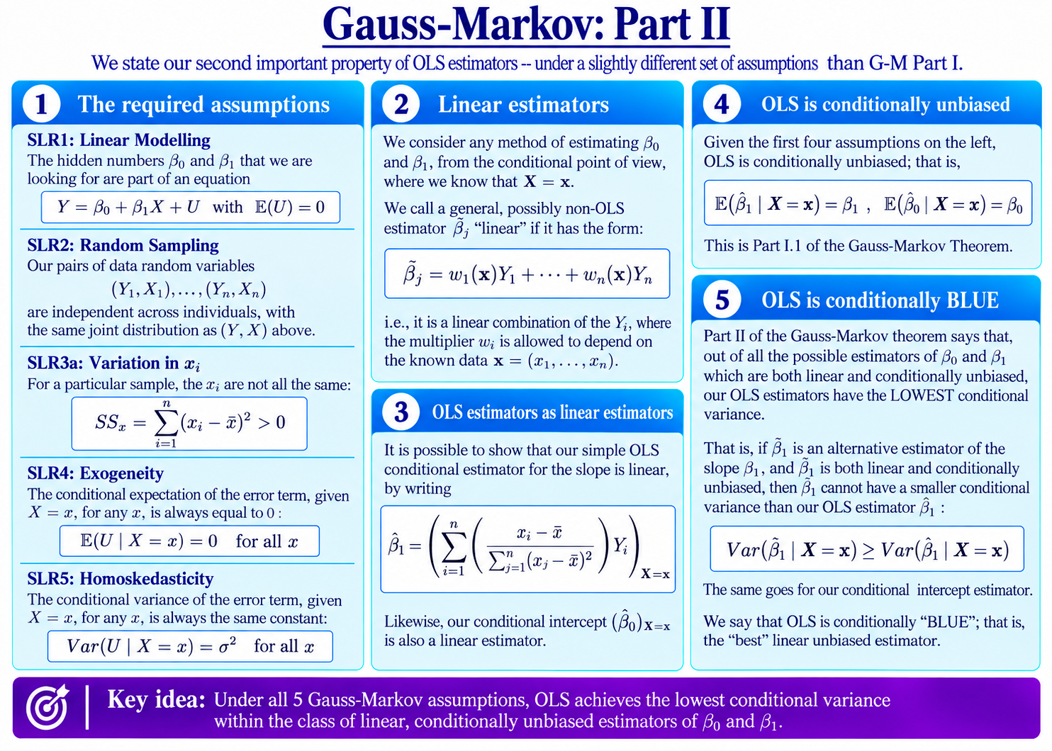
Gauss-Markov: Part II

We have already established one major result about OLS.

Under SLR1, SLR2, SLR3a and SLR4, OLS is conditionally unbiased:

$$\mathbb{E}(\hat\beta_1\mid\mathbf{X}=\mathbf{x})=\beta_1$$

and

$$\mathbb{E}(\hat\beta_0\mid\mathbf{X}=\mathbf{x})=\beta_0$$

We now add our final Gauss-Markov assumption, SLR5: Homoskedasticity.

This gives us something more: efficiency.

Among a particular class of alternative estimators that are also conditionally unbiased, clarified below, OLS has the lowest conditional variance.

The Required Assumptions

For this result, we use all five of our Gauss-Markov assumptions.

SLR1: Linear Modelling

$$Y=\beta_0+\beta_1X+U,\qquad \mathbb{E}(U)=0$$

SLR2: Random Sampling

$$(Y_1,X_1),\ldots,(Y_n,X_n)\ \text{are i.i.d. copies of }(Y,X)$$

SLR3a: Variation in the Observed $x_i$

$$SS_x=\sum_{i=1}^{n}(x_i-\bar{x})^2>0$$

SLR4: Exogeneity

$$\mathbb{E}(U\mid X=x)=0\qquad\text{for all }x$$

SLR5: Homoskedasticity

$$\operatorname{Var}(U\mid X=x)=\sigma^2\qquad\text{for all }x$$

What Is a Linear Estimator?

Before stating the theorem precisely, we need to say which alternative estimators OLS is competing against when we say it is the “best one”.

We work from our usual conditional point of view, where

$$\mathbf{X}=\mathbf{x}=(x_1,\ldots,x_n)$$

has already been observed.

We call an estimator of $\beta_j$ linear if it can be written in the form

$$\tilde\beta_j=w_1(\mathbf{x})Y_1+\cdots+w_n(\mathbf{x})Y_n$$

for some weights $w_1(\mathbf{x}),\ldots,w_n(\mathbf{x})$.

So, we multiply each $Y_i$ by some weight, then add the results together.

As the notation indicates, weights are allowed to depend on the known $\mathbf{x}=(x_1,\dots,x_n)$. However, the estimator must be a linear combination of the $Y_i$: we cannot start doing more exotic things such as squaring them, taking their square roots, or multiplying them together.

For example, the sample mean

$$\bar{Y}=\frac{1}{n}Y_1+\cdots+\frac{1}{n}Y_n$$

is a linear estimator, with every weight equal to $1/n$.

OLS Is a Linear Estimator

Our OLS slope estimator belongs to this class too.

From the conditional point of view,

$$\hat\beta_1=\frac{\sum_{i=1}^{n}(x_i-\bar{x})(Y_i-\bar{Y})}{\sum_{i=1}^{n}(x_i-\bar{x})^2}$$

Using our usual disappearing-mean trick,

$$\hat\beta_1=\frac{\sum_{i=1}^{n}(x_i-\bar{x})Y_i}{\sum_{i=1}^{n}(x_i-\bar{x})^2}$$

and hence

$$\hat\beta_1=\sum_{i=1}^{n}\left(\frac{x_i-\bar{x}}{\sum_{j=1}^{n}(x_j-\bar{x})^2}\right)Y_i$$

So OLS simply uses the weights

$$w_i(\mathbf{x})=\frac{x_i-\bar{x}}{\sum_{j=1}^{n}(x_j-\bar{x})^2}$$

The intercept estimator is linear too. Since

$$\hat\beta_0=\bar{Y}-\bar{x}\hat\beta_1$$

we can write

$$\hat\beta_0=\sum_{i=1}^{n}\left(\frac{1}{n}-\frac{\bar{x}(x_i-\bar{x})}{\sum_{j=1}^{n}(x_j-\bar{x})^2}\right)Y_i$$

So both of our OLS estimators are linear estimators.

The Competition

Now consider some alternative estimator of the slope, with a different choice of weights:

$$\tilde\beta_1=w_1(\mathbf{x})Y_1+\cdots+w_n(\mathbf{x})Y_n$$

Suppose that this estimator satisfies two conditions.

First, it is linear, in the sense just described.

Second, it is conditionally unbiased:

$$\mathbb{E}(\tilde\beta_1\mid\mathbf{X}=\mathbf{x})=\beta_1$$

OLS itself satisfies both conditions. The key question is then:

Could $\tilde\beta_1$ give us an unbiased estimator with a smaller conditional variance than OLS?

Gauss-Markov: Part II

Under SLR1, SLR2, SLR3a, SLR4 and SLR5, the answer to our key question is a resounding “no”.

For any linear, conditionally unbiased estimator $\tilde\beta_1$ of $\beta_1$,

$$\operatorname{Var}(\tilde\beta_1\mid\mathbf{X}=\mathbf{x})\geq\operatorname{Var}(\hat\beta_1\mid\mathbf{X}=\mathbf{x})$$

Likewise, for any linear, conditionally unbiased estimator $\tilde\beta_0$ of $\beta_0$,

$$\operatorname{Var}(\tilde\beta_0\mid\mathbf{X}=\mathbf{x})\geq\operatorname{Var}(\hat\beta_0\mid\mathbf{X}=\mathbf{x})$$

So, amongst all the linear and conditionally unbiased estimators, OLS has the smallest possible conditional variance.

That is the second major part of the Gauss-Markov theorem.

OLS is “BLUE”

In investigating our simple line of best fit approach, we have managed to accumulate rather a lot of adjectives.

Fortunately, by a huge stroke of luck, the four adjectives we need here are easier to remember since they happen to spell the name of a colour:

Best Linear Unbiased Estimator – BLUE.

Each word matters.

Best means having the lowest conditional variance amongst the estimators in the comparison.

Linear means being a weighted linear combination of the $Y_i$.

Unbiased here means conditionally unbiased, given $\mathbf{X}=\mathbf{x}$.

And Estimator means that we are using our sample data to estimate the unknown coefficients $\beta_0$ and $\beta_1$.

So, under the five Gauss-Markov assumptions, OLS is conditionally BLUE.

Notice that Gauss-Markov does not say that OLS has the lowest conditional variance amongst every conceivable unbiased estimator. More exotic, non-linear estimators are simply outside the competition. There is a further, sixth assumption that does guarrantee this; but we’ll come back to this later on the next pass, when we cover multiple regression.

Proving the Result for the OLS Slope

Let’s finish this section of slides by tackling the final boss: the proof of Gauss-Markov Part II for $\hat\beta_1$. We do the proof in five steps.

Step I: Characterising Unbiased estimators

Consider any linear estimator

$$\tilde\beta_1=\sum_{i=1}^{n}w_i(\mathbf{x})Y_i$$

We want this estimator to be conditionally unbiased. Taking a conditional expectation:

$$ \mathbb{E}(\tilde\beta_1 \mid \mathbf{X}=\mathbf{x}) = \mathbb{E} \left( \sum_{i=1}^{n} w_i(\mathbf{x})Y_i\mid\mathbf{X}=\mathbf{x} \right) $$

From the conditional point of view, the $x_i$ and hence the weights $w_i(\mathbf{x})$ are fixed. Bringing these out, and splitting up the expectation, gives:

$$ = \sum_{i=1}^{n} w_i(\mathbf{x})\mathbb{E}(Y_i\mid\mathbf{X}=\mathbf{x} ) $$

Using SLR1, SLR2 and SLR4, we have $\mathbb{E}(Y_i\mid\mathbf{X}=\mathbf{x})=\beta_0+\beta_1x_i$. So, we obtain:

$$=\sum_{i=1}^{n}w_i(\mathbf{x})(\beta_0+\beta_1x_i)$$

Expanding,

$$=\beta_0\sum_{i=1}^{n}w_i(\mathbf{x})+\beta_1\sum_{i=1}^{n}w_i(\mathbf{x})x_i$$

For this to equal $\beta_1$ regardless of the particular unknown values of $\beta_0$ and $\beta_1$, we need

$$\sum_{i=1}^{n}w_i(\mathbf{x})=0$$

and

$$\sum_{i=1}^{n}w_i(\mathbf{x})x_i=1$$

So these are the two restrictions on our weights required for conditional unbiasedness. For readability, let’s drop the dependence on $\mathbf{x}$ and write $w_i(\mathbf{x})=w_i$.

Step II: A General Conditional Variance

We now ask which weights satisfying those two restrictions produce the smallest conditional variance.

Taking the conditional variance, we have

$$\operatorname{Var}(\tilde\beta_1\mid\mathbf{X}=\mathbf{x})=\operatorname{Var}\left(\sum_{i=1}^{n}w_iY_i\mid\mathbf{X}=\mathbf{x}\right)$$

From SLR2, the $Y_i$ are independent, even conditional on $\mathbf{X}=\mathbf{x}$, and we can split up the variance. Moreover, for $Y_i$, conditioning on $X_j$ has no effect for $j≠i$:

$$= \sum_{i=1}^{n}\operatorname{Var}(w_iY_i \mid X_i = X_i )$$

Bringing the fixed terms out:

$$=\sum_{i=1}^{n}w_i^2\operatorname{Var}(Y_i\mid X_i = x_i )$$

Using SLR1 and SLR2:

$$=\sum_{i=1}^{n}w_i^2\operatorname{Var}(\beta_0 + \beta_1X_i + U_i \mid X_i=x_i)$$

Removing the fixed terms again:

$$=\sum_{i=1}^{n}w_i^2\operatorname{Var}(U_i \mid X_i=x_i)$$

From SLR2 and SLR5, homoskedasticity, we have:

$$=\sum_{i=1}^{n}w_i^2 \sigma^2 $$

That is:

$$=\sigma^2\sum_{i=1}^{n}w_i^2$$

Step III: Finding the Minimum

Since $\sigma^2$ is fixed, minimising the conditional variance is therefore equivalent to solving

$$\min_{w_1,\ldots,w_n}\sum_{i=1}^{n}w_i^2$$

subject to

$$\sum_{i=1}^{n}w_i=0$$

and

$$\sum_{i=1}^{n}w_ix_i=1$$

We have turned the Gauss-Markov theorem into a constrained optimisation problem!

We tackle this using the standard Lagrangian method.

Write

$$L=\sum_{i=1}^{n}w_i^2-\lambda\sum_{i=1}^{n}w_i-\mu\left(\sum_{i=1}^{n}w_ix_i-1\right)$$

We now find the first-order conditions.

For a generic weight $w_i$,

$$\frac{\partial L}{\partial w_i}=2w_i-\lambda-\mu x_i=0$$

so

$$w_i=\frac{1}{2}(\lambda+\mu x_i)$$

We now use the two unbiasedness restrictions to find $\lambda$ and $\mu$.

Step IV: Finding $\lambda$ and $\mu$

First, we require

$$\sum_{i=1}^{n}w_i=0$$

Substituting our expression for $w_i$,

$$\sum_{i=1}^{n}\frac{1}{2}(\lambda+\mu x_i)=0$$

so

$$\frac{n}{2}\lambda+\frac{\mu}{2}\sum_{i=1}^{n}x_i=0$$

Since

$$\sum_{i=1}^{n}x_i=n\bar{x}$$

we obtain

$$\lambda=-\mu\bar{x}$$

Next, use our second restriction:

$$\sum_{i=1}^{n}w_ix_i=1$$

Substituting again,

$$\sum_{i=1}^{n}\frac{1}{2}(\lambda+\mu x_i)x_i=1$$

and therefore

$$\lambda\sum_{i=1}^{n}x_i+\mu\sum_{i=1}^{n}x_i^2=2$$

Using $\lambda=-\mu\bar{x}$,

$$\mu\left(\sum_{i=1}^{n}x_i^2-\bar{x}\sum_{i=1}^{n}x_i\right)=2$$

But

$$\sum_{i=1}^{n}x_i^2-\bar{x}\sum_{i=1}^{n}x_i=\sum_{i=1}^{n}(x_i-\bar{x})^2=SS_x$$

so

$$\mu=\frac{2}{SS_x}$$

and therefore

$$\lambda=-\frac{2\bar{x}}{SS_x}$$

Step V: The OLS Weights Appear

Finally, substitute these values back into

$$w_i=\frac{1}{2}(\lambda+\mu x_i)$$

We get

$$w_i=\frac{1}{2}\left(-\frac{2\bar{x}}{SS_x}+\frac{2x_i}{SS_x}\right)$$

and hence

$$w_i=\frac{x_i-\bar{x}}{SS_x}$$

or, writing out $SS_x$,

$$w_i=\frac{x_i-\bar{x}}{\sum_{j=1}^{n}(x_j-\bar{x})^2}$$

But these are exactly the weights used by the OLS slope estimator!

Since our objective $\sum_{i=1}^{n}w_i^2$ is convex and the restrictions are linear, this solution gives the minimum.

So the choice of weights that gives the smallest possible conditional variance, whilst preserving conditional unbiasedness, is precisely the OLS choice.

Therefore $\hat\beta_1$ is the best linear unbiased estimator of $\beta_1$.

A similar argument establishes the result for $\hat\beta_0$.

If you followed all of this, you have my permission to reward yourself with a night out down the pub, should you choose to do so.

Background

• Variance and Standard Deviation
• Properties of Variance and Covariance
• Conditional Expectations
• Conditional Variance and the Law of Total Variance
• Unbiasedness
• Efficiency
• Conditioning on X
• SLR1: Linear Modelling
• SLR2: Random Sampling
• SLR3: Variation in X
• SLR4: Exogeneity
• Gauss-Markov – Part I
• SLR5: Homoskedasticity
• Variance of OLS Estimators in a SLR
• Lagrange Worked Example