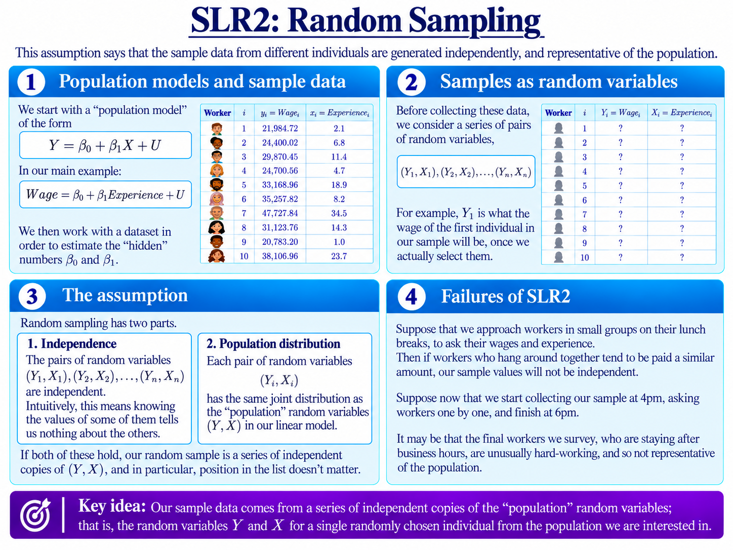
The Random Sampling Assumption

Our second assumption concerns how the data used in our regression are generated.

As we know, our overall goal is to estimate the coefficients $\beta_0$ and $\beta_1$ in the linear model:

$$Y=\beta_0+\beta_1X+U.$$

To do so, we collect some data on $Y$ and $X$, our population random variables. In our main example, these represent the wage and experience of a randomly chosen worker from the population we are interested in.

Of course, we will not collect data from just one randomly chosen worker. Rather, we collect a whole sample of observations comprising $n$ individuals.

SLR2: Random Sampling says that the pairs of random variables

$$(Y_1,X_1),(Y_2,X_2),\ldots,(Y_n,X_n)$$

are independent, and that each pair $(Y_i,X_i)$ has the same joint distribution as the population pair $(Y,X)$.

That is, our $(Y_i,X_i)$ are independent and identically distributed, or i.i.d., copies of $(Y,X)$.

We introduced the general idea of a random sample earlier in the statistics section. The only difference here is that each “observation” now has both an outcome and an independent variable.

We unpack this in a little more detail below, and see why it might fail.

Before and After Collecting the Sample

Suppose that we plan to collect data from $n$ workers.

Before collecting the data, $Y_1$ represents the wage of the first worker who will enter our sample, while $X_1$ represents their experience. At this stage these quantities are still random variables: we do not yet know which workers we will select, or what their wages and experience levels will be.

Once the sample has actually been collected, they become the observed numbers

$$(y_1,x_1),(y_2,x_2),\ldots,(y_n,x_n).$$

SLR2 places two requirements on the pairs of random variables $(Y_i,X_i)$ from which these observations arise.

Part 1: Independence

First, the pairs must be independent.

Intuitively, knowing the values taken by some observations should give us no information about the values taken by the others.

For example, suppose that we approach workers in small groups during their lunch breaks. If workers who spend their breaks together also tend to have similar wages, then observations collected from the same group may be related.

In that case, learning about one worker would tell us something about another, and the independence part of SLR2 would fail.

Note that we are not, of course, saying that $Y_i$ and $X_i$ are independent of each other; rather, that the pairs of data from different workers are independent.

Now, as we did on the SLR1: Linear Modelling page, for the numbers $\beta_0$ and $\beta_1$ we are seeking, we can define the error term:

$$U_i=Y_i-\beta_0-\beta_1X_i.$$

Then, since $U_i$ is a combination of $Y_i$ and $X_i$, it follows automatically that the triples $(Y_i,X_i,U_i)$ are independent too – that is, across different workers (not within individual triples).

Part 2: The Population Distribution

Second, each pair $(Y_i,X_i)$ must have the same joint distribution as the population pair $(Y,X)$.

This means that every position in our sample represents another draw from the same population we are trying to study.

In particular, there is nothing special about being worker 1, worker 7 or worker $n$. Before the data are collected, every position in the sample plays the same probabilistic role.

As an example of this going wrong, suppose that we begin surveying workers at 4pm and continue until 6pm. Workers still at work later in the evening might be more hard-working or committed, or occupy more senior roles; they might therefore tend to have a higher wage than the average for the broader population of workers.

In this case, position in the list does matter: the wages of workers towards the end of our sample have a different distribution. Our observations would therefore not all be representative of the population, and SLR2 would fail.

As before, this second part of SLR2 also extends automatically to the error term. Since we have both

$$U=Y-\beta_0-\beta_1X$$

and

$$U_i=Y_i-\beta_0-\beta_1X_i,$$

if $(Y_i,X_i)$ has the same joint distribution as $(Y,X)$, then $U_i$ has the same distribution as $U$.

Finally, putting both parts of SLR2 together, the triples $(Y_i,X_i,U_i)$ are independent copies of the population triple $(Y,X,U)$.

The Importance of SLR2

Mathematically, the importance of SLR2 is as follows.

The first part, independence, will be useful because in our later proofs we will need to work with independent random variables – especially when handling the error terms $U_i$.

Meanwhile, the second part of SLR2 has an important role in extending other properties we assume about the population random variables to our sample.

For instance, suppose that SLR1: Linear Modelling also holds. Then we have

$$\mathbb{E}(U)=0.$$

But since $U_i \sim U$, from SLR2, it follows immediately that

$$\mathbb{E}(U_i)=0.$$

From a practical point of view, SLR2 says that we have collected our data sensibly. In advanced topics, we consider what happens when this fails.

Background

• Independence
• Random Samples
• SLR1: Linear Modelling