Three Perspectives

In the previous slide, we introduced the idea of evaluating OLS using probability and statistics.

Before we get going with this process, however, we need one final important distinction: the idea of conditioning on $X$.

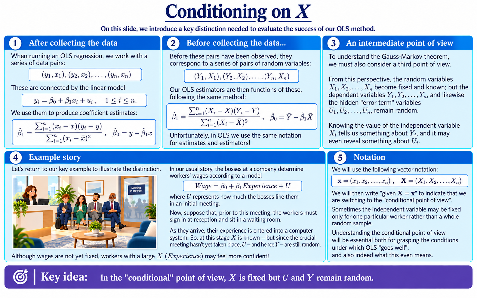
Probability and statistics already require us to move fluently between two different points of view. Before collecting our data, we work with random variables whose values are not yet known. From this perspective, we use the tools of the theory of probability. After collecting the data, however, we work with particular values that have actually been observed, which must now be treated as fixed numbers.

In econometrics, it is also useful to consider a third, intermediate perspective. That is: we treat the values of the independent variable $X$ as fixed, while the error term $U$ and dependent variable $Y$ remain random.

This is the conditional point of view.

The first two perspectives should already be familiar. The third may be known to you if you’ve looked at conditioning in detail. It plays a central role in both the Gauss-Markov assumptions and in what it means for OLS to work well.

Perspective 1. After Collecting the Data

Once we have collected our sample, we have a list of observed data pairs:

$$(y_1,x_1),\ (y_2,x_2),\ \dots,\ (y_n,x_n).$$

These are simply numbers.

For each observation, our simple linear model gives

$$y_i=\beta_0+\beta_1x_i+u_i,\qquad i=1,\dots,n.$$

Here $u_i$ is also now a fixed number, although unlike $x_i$ and $y_i$ it will generally be hidden from us.

Using the observed data, we calculate our OLS estimates:

$$\hat\beta_1=\frac{\sum_{i=1}^{n}(x_i-\bar{x})(y_i-\bar{y})}{\sum_{i=1}^{n}(x_i-\bar{x})^2},\qquad \hat\beta_0=\bar{y}-\hat\beta_1\bar{x}.$$

At this stage, the data have already been observed. The OLS estimates $\hat\beta_0$ and $\hat\beta_1$ are therefore just numerical values too.

Perspective 2. Before Collecting the Data

Before the sample has been observed, the situation looks different.

For each position $i$ within our future sample, we instead work with random variables

$$(Y_i,X_i,U_i),$$

connected by our linear model,

$$Y_i=\beta_0+\beta_1X_i+U_i.$$

At this stage, $X_i$, $Y_i$ and $U_i$ are random variables: their particular realised values have not yet been observed.

Likewise, our OLS estimators are random variables:

$$\hat\beta_1=\frac{\sum_{i=1}^{n}(X_i-\bar{X})(Y_i-\bar{Y})}{\sum_{i=1}^{n}(X_i-\bar{X})^2},\qquad \hat\beta_0=\bar{Y}-\hat\beta_1\bar{X}.$$

This is because their values depend on the data we are yet to obtain, so they are also at present uncertain. As random variables, we can ask, for example, interesting questions about their expectations and variances.

Perspective 3. Conditioning on $X$

Now for the third point of view!

We consider the random variables for our independent variable, one at each position within our sample:

$$X_1,\dots,X_n$$

Now, suppose we fix these at some particular values:

$$x_1,\dots,x_n.$$

However, the error terms $U_1,\dots,U_n$ remain random, and the corresponding dependent variables $Y_1,\dots,Y_n$ remain random too.

This is what we mean by conditioning on $X$.

It is useful to introduce some compact notation. Let

$$\mathbf{X}=(X_1,\dots,X_n),\qquad \mathbf{x}=(x_1,\dots,x_n).$$

We can then write

$$\mathbf{X}=\mathbf{x}$$

to indicate that the whole collection of $X$-values is being treated as fixed.

To recap: from this conditional point of view, the $x_i$ now become constants, while the $U_i$ and $Y_i$ remain random. Importantly, since our OLS estimators depend on $Y_i$, these remain random too.

Why Is This Useful?

Conditioning on $X$ makes many questions about OLS easier, and is essential even for stating others.

In particular, it is what allows us to study quantities such as the conditional expectation:

$$\mathbb{E}(\hat\beta_1\mid\mathbf{X}=\mathbf{x})$$

and the conditional variance:

$$\operatorname{Var}(\hat\beta_1\mid\mathbf{X}=\mathbf{x}).$$

As we’ll see shortly, these ideas will play a central role in the Gauss-Markov theorem.

An Intuition from Our Main Example

Returning to our running example, we can give this somewhat abstract idea a particularly concrete interpretation.

Recall that we were imagining some workers whose wages were determined by the formula

$$Wage=\beta_0+\beta_1Experience+U,$$

where $U$ represents how much the bosses like a worker when they meet them at an initial meeting.

Suppose the workers we have randomly selected for our sample arrive at reception before their interviews. Upon arrival, their levels of experience are already entered into a computer system. So, if we were to check the system, the values of $X_i$ would now be observable to us.

At this stage, however, the workers have not yet met the bosses – so the values of $U_i$ are still uncertain. And since their eventual wages depend on $U$, their values of $Y$ are still random too.

However, something has changed: given the $X_i$, we may now have certain expectations about $Y_i$. That is, those who have more experience are now likely – though perhaps not certain – to receive a higher wage overall.

Moreover, depending on the nature of the situation, knowing $X$ may (or may not) give us an inkling about whether the workers are likely to do well at the interview, too!

Background

• Random Variables
• Conditional Expectations
• Conditional Variance and the Law of Total Variance
• Estimators as Random Variables
• OLS Estimation
• Evaluating OLS: Gauss-Markov