What Is an Estimator?

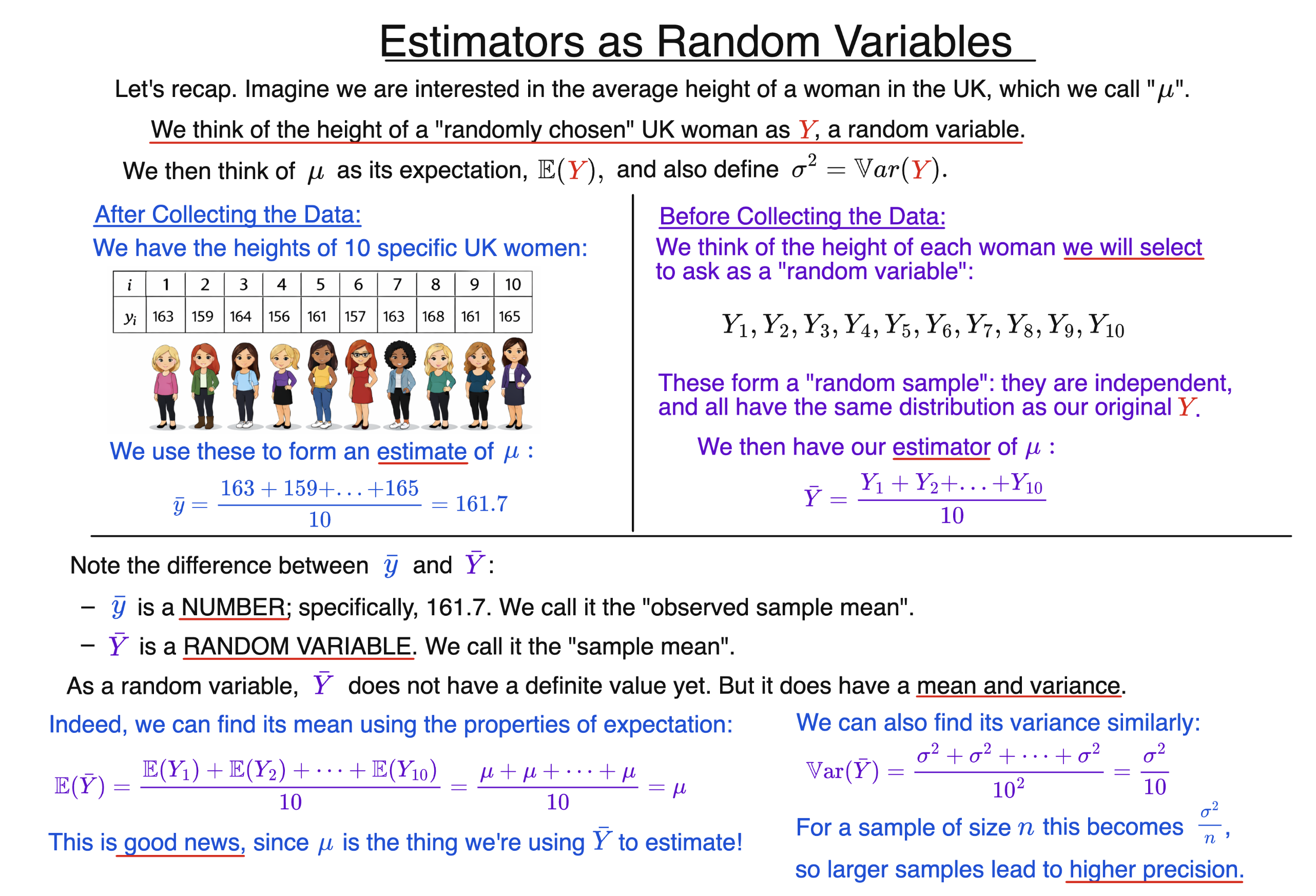
Intuitively, an estimator is a random variable which we use to estimate an unknown quantity. It is formed from a random sample, such as

$$Y_1,Y_2,\dots,Y_n.$$

More precisely, an estimator is a function of these $Y_1,Y_2,\dots,Y_n$, which we happen to use in this way. Such a function is called a statistic — the same as the name of the subject itself!

In our main example, the random variables $Y_1,Y_2,\dots,Y_n$ represent the heights of $n$ women we are planning to select at random from the UK population. They are random because we have not yet selected the women — just as the outcome of a die roll is random before we actually roll the die.

Given some observed data

$$y_1,y_2,\dots,y_n,$$

it is natural to estimate the population average height by taking their average:

$$\bar y=\frac{y_1+y_2+\dots+y_n}{n}.$$

This is the observed sample mean. Once the data have been collected, $\bar y$ is simply a number: an estimate of the population mean $\mu$.

The corresponding estimator looks almost the same, but uses the random variables $Y_i$ rather than the observed numbers $y_i$:

$$\bar Y=\frac{Y_1+Y_2+\dots+Y_n}{n}.$$

This random variable $\bar Y$ is called the sample mean. It is an important example of an estimator, and we commonly use it to estimate

$$\mu=\mathbb{E}(Y_i).$$

The distinction between these two things is very important:

• $\bar y$ is an estimate: a number obtained after collecting our data.
• $\bar Y$ is an estimator: a random variable that exists before we collect our data.

Sometimes we think of an estimator as a formula or “method” for producing an estimate from a dataset. But we should also be conscious that it is a random variable in its own right, just like the individual $Y_i$.

This means that we can investigate estimators using probability theory.

Estimators Have Means and Variances

Since an estimator such as $\bar Y$ is a random variable, it has an expected value and a variance. We can find these using our two key properties of random samples: independence, and being identically-distributed.

For a random sample, each $Y_i$ has the same expected value, $\mu$. So, using the properties of expectation,

$$\mathbb{E}(\bar Y)=\mathbb{E}\left(\frac{Y_1+Y_2+\dots+Y_n}{n}\right)=\frac{\mathbb{E}(Y_1)+\mathbb{E}(Y_2)+\dots+\mathbb{E}(Y_n)}{n}=\frac{\mu+\mu+\dots+\mu}{n}=\mu.$$

We note that this is the same number we are using $\bar Y$ to estimate. This is encouraging!

Meanwhile, since the random variables in our random sample are independent, we can also find the variance:

$$\operatorname{Var}(\bar Y)=\operatorname{Var}\left(\frac{Y_1+Y_2+\dots+Y_n}{n}\right)=\frac{\operatorname{Var}(Y_1)+\operatorname{Var}(Y_2)+\dots+\operatorname{Var}(Y_n)}{n^2}.$$

Since each $Y_i$ has variance $\sigma^2$,

$$\operatorname{Var}(\bar Y)=\frac{\sigma^2+\sigma^2+\dots+\sigma^2}{n^2}=\frac{\sigma^2}{n}.$$

So the distribution of our estimator becomes less “spread out” as the sample size gets larger.

In other words, larger samples give us greater precision — which is generally something we should feel pleased about.

Background

• Random Variables

• Expected Values

• Variance and Standard Deviation

Extensions

• Unbiasedness

• Efficiency