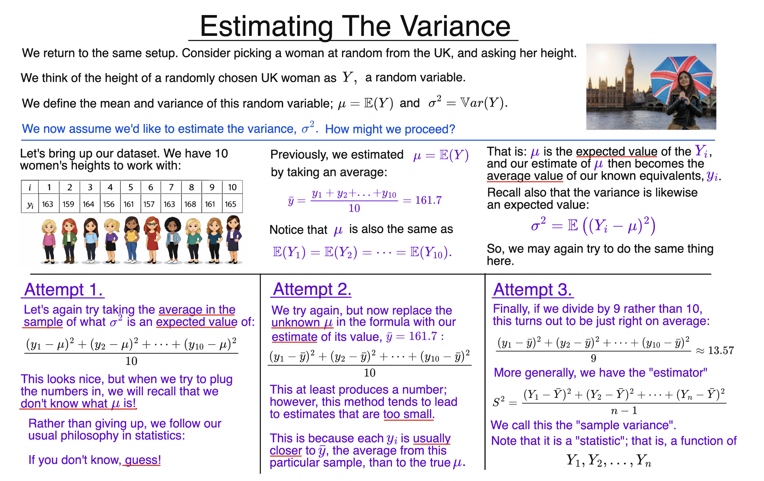
How Do We Estimate the Variance?

Suppose we would like to know the variance of a certain population; for instance, the variance of women’s heights in the UK.

We think of the height of a woman we will randomly select from the UK population as a random variable $Y$, and the population variance we want to find as

$$\sigma^2=\operatorname{Var}(Y).$$

Given some data

$$y_1,y_2,\dots,y_n,$$

how could we estimate $\sigma^2$?

We already know how to estimate the population mean $\mu$. The idea is to take the average of our random sample:

$$\bar Y=\frac{Y_1+Y_2+\dots+Y_n}{n}.$$

We will now try to extend the same basic idea to the variance.

Attempt 1: Take an Average

Recall that variance can itself be written as an expected value:

$$\sigma^2=\mathbb{E}\left((Y-\mu)^2\right).$$

So it seems natural to estimate it by taking the average value of $(Y_i-\mu)^2$ across our random sample:

$$\frac{(Y_1-\mu)^2+(Y_2-\mu)^2+\dots+(Y_n-\mu)^2}{n}.$$

There is just one rather serious problem: this is not an estimator.

An estimator must be a statistic; that is, a function of the underlying random sample $Y_1,Y_2,\dots,Y_n$. But the expression above also depends on the unknown population mean $\mu$.

Even after collecting our data and turning $Y_1,Y_2,\dots,Y_n$ into the observed numbers $y_1,y_2,\dots,y_n$, we still could not calculate its value, because we still would not know $\mu$.

So it is no use for producing estimates in practice.

Still, this was a good start, and we needn’t be discouraged. If you don’t know, guess!

Attempt 2: Replace $\mu$ With the Sample Mean

We do not know $\mu$, but we do have an estimator of it: the sample mean $\bar Y$.

So let’s try replacing $\mu$ with $\bar Y$:

$$\frac{(Y_1-\bar Y)^2+(Y_2-\bar Y)^2+\dots+(Y_n-\bar Y)^2}{n}.$$

This is now a genuine estimator, since it is entirely a function of the random sample.

Unfortunately, there is another issue with it, albeit a less serious one: it tends to be too small on average.

The intuition for this is that $\bar Y$ has been calculated from the very same observations whose deviations from the mean we are trying to measure. The sample observations therefore tend to lie closer to their own sample mean than they do to the true population mean.

Suppose, for example, that the women in a particular sample just happen to be rather tall on the whole. Then $\bar y$ will be larger than $\mu$. The squared deviations

$$(y_i-\bar y)^2$$

will tend to be smaller than the corresponding squared deviations from the true population mean,

$$(y_i-\mu)^2.$$

By replacing the unknown $\mu$ with the sample mean $\bar Y$, we have therefore made our estimator of $\sigma^2$ slightly too small on average.

Attempt 3: Divide by $n-1$

The correction to this problem turns out to be remarkably neat: instead of dividing by $n$, we divide by $n-1$.

This gives the sample variance estimator:

$$S_n^2=\frac{(Y_1-\bar Y)^2+(Y_2-\bar Y)^2+\dots+(Y_n-\bar Y)^2}{n-1}.$$

With this correction, $S_n^2$ is neither systematically too large nor too small on average. That is,

$$\mathbb{E}(S_n^2)=\sigma^2.$$

This property, shared by the sample mean, is called unbiasedness. We cover it in more detail later.

One common way of thinking about the appearance of $n-1$ in particular here is in terms of degrees of freedom.

Once we have used the sample to estimate the unknown population mean $\mu$ by $\bar Y$, the deviations

$$Y_1-\bar Y,\ Y_2-\bar Y,\dots,Y_n-\bar Y$$

must add up to zero. So, now only $n-1$ of these deviations can vary freely. In this sense, the introduction of $\bar Y$ has “used up” one degree of freedom. Essentially, this means that the overall sum of squared deviations behaves more like a quantity with $n-1$ squared terms rather than $n$! This suggests that we should divide by $n-1$ rather than $n$.

This probably all sounds very mysterious, but explaining degrees of freedom properly will have to wait for another time. A little later on this page, however, we give a mathematical proof that dividing by $n-1$ really does produce the result above.

From the Estimator to an Estimate

Once we have actually collected the data, we replace the random variables $Y_i$ with the observed numbers $y_i$.

For the $10$ women’s heights on the slide, the observed sample mean is

$$\bar y=161.7.$$

The corresponding sample variance is

$$\frac{(163-161.7)^2+(159-161.7)^2+\dots+(165-161.7)^2}{9}\approx13.57.$$

So our estimate of the population variance $\sigma^2$ is approximately

$$13.57.$$

Estimating the Standard Deviation

If we want to estimate the population standard deviation

$$\sigma=\sqrt{\operatorname{Var}(Y)},$$

the natural thing to do is take the square root of the sample variance:

$$S_n=\sqrt{S_n^2}=\sqrt{\frac{(Y_1-\bar Y)^2+(Y_2-\bar Y)^2+\dots+(Y_n-\bar Y)^2}{n-1}}.$$

We should remember that $S_n^2$ is defined first, and $S_n$ is just its square root.

Also, although

$$\mathbb{E}(S_n^2)=\sigma^2,$$

this does not imply that

$$\mathbb{E}(S_n)=\sigma.$$

Taking a square root does not generally commute with taking an expectation.

Proof of Bessel’s Correction

We can now prove that dividing by $n-1$ gives an unbiased estimator of $\sigma^2$.

We use the identity

$$\sum_{i=1}^n(Y_i-\bar Y)^2=\sum_{i=1}^n(Y_i-\mu)^2-n(\bar Y-\mu)^2.$$

Taking expectations, the first term on the right contributes

$$n\sigma^2,$$

since each $Y_i$ has variance $\sigma^2$.

Meanwhile, since $\mathbb{E}(\bar Y)=\mu$,

$$\mathbb{E}\left((\bar Y-\mu)^2\right)=\operatorname{Var}(\bar Y).$$

Using the independence of the random variables in our random sample,

$$\operatorname{Var}(\bar Y)=\frac{\sigma^2}{n}.$$

Therefore,

$$\mathbb{E}\left(\sum_{i=1}^n(Y_i-\bar Y)^2\right)=n\sigma^2-n\frac{\sigma^2}{n}=(n-1)\sigma^2.$$

Dividing by $n-1$ gives

$$\mathbb{E}(S_n^2)=\sigma^2.$$

So the $n-1$ correction does exactly what we claimed.

An Equivalent Formula

Finally, an equivalent formula for the sample variance is often easier to work with:

$$S_n^2=\frac{(Y_1^2+Y_2^2+\dots+Y_n^2)-n\bar Y^2}{n-1}.$$

This gives exactly the same estimator as the formula using squared deviations from the sample mean.

Background

• Variance and Standard Deviation

Extensions

• Unbiasedness