Ordinary Least Squares

We are now finally ready to make our idea of a line of best fit mathematically precise.

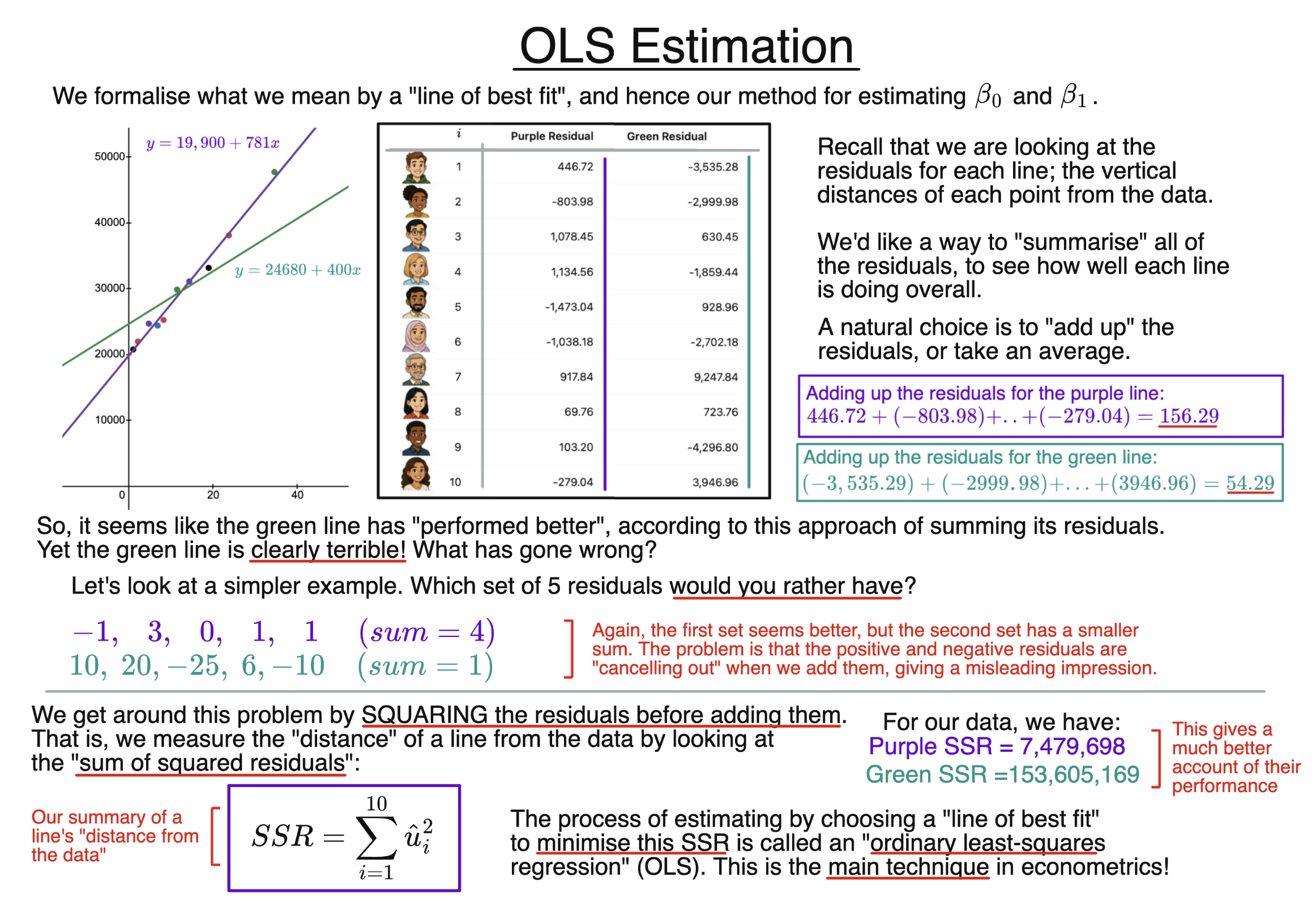
For any candidate line, we can calculate a residual for each observation: the vertical difference between the observed value $y_i$ and the fitted value on the line.

We would like these residuals to be “small overall”, so we need a summary of what this means.

We might at first think of simply adding them, or taking an average. However, as it turns out, this is not a good method to measure the fit of the line.

As shown by example in the slide, the problem is that positive and negative residuals can cancel each other out, sometimes making a badly fitting line appear much better than it really is.

We need a way to prevent this cancelling out from happening. If you thought of taking the absolute values of the residuals – then congratulations, you just reinvented “LAD” regression! This is a little less exciting than it sounds (LAD = “least absolute deviations”), and in any case is not how we usually do things around here.

Instead, we will prevent cancellations by squaring the residuals before adding them together.

This should remind us of the definition of the variance, where we squared the difference between $X$ and $\mu$, because otherwise we had

$$\mathbb{E}(X-\mu)=\mathbb{E}(X)-\mu=\mu-\mu=0.$$

The Sum of Squared Residuals

Recall that for our final fitted line, the residual for observation $i$ is

$$\hat u_i=y_i-\hat y_i.$$

We define the sum of squared residuals, or SSR, as

$$SSR=\sum_{i=1}^{n}\hat u_i^2.$$

Since a square cannot be negative, squaring removes the problem of positive and negative residuals cancelling out.

A smaller $SSR$ therefore indicates that the line fits our data better.

Another consequence of squaring is that particularly large residuals contribute especially heavily to the total. For instance, $12$ is four times as large as $3$; but if we square both values, $12^2$ is now sixteen times as large as $3^2$, and therefore has relatively more influence on our measure of fit.

OLS Estimation

We have arrived at our key method for linear regression: Ordinary Least Squares – usually abbreviated to OLS. That is, we choose the line whose sum of squared residuals is as small as possible.

Of course, the name “least squares” comes from the idea of minimising the $SSR$, and we say “ordinary” because that’s how we ordinarily do things. Indeed, even much more advanced modern methods in econometrics are usually just “OLS with extra steps”!

So, to reiterate, amongst all the possible straight lines we could draw through the data, OLS chooses the intercept and slope that minimise the SSR.

The resulting line is our line of best fit:

$$\hat y_i=\hat\beta_0+\hat\beta_1x_i.$$

Its intercept $\hat\beta_0$ and slope $\hat\beta_1$ are therefore our OLS estimates of the unknown coefficients $\beta_0$ and $\beta_1$ in the original linear model.

This is what we mean, mathematically, when we say that we “run a linear regression”.

Background

• Variance and Standard Deviation
• Estimands, Estimates, and Estimators
• Residuals vs Errors
• Lines of Best Fit