Evaluating the Method

In previous slides, we have produced some encouraging empirical results. But we would now like to evaluate the reliability of OLS more carefully, using the formal tools of probability and statistics.

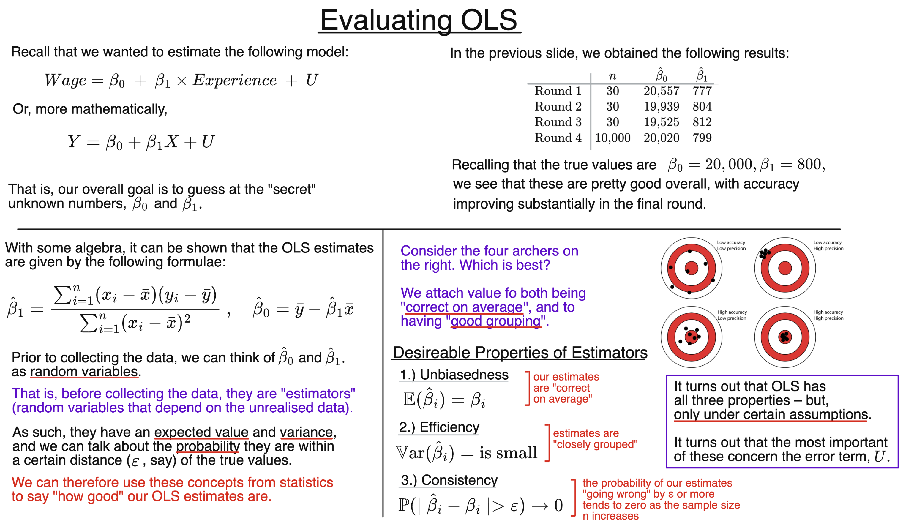
OLS is a precise, maths-based method that can be repeated exactly. So, rather than having to work out the line of best fit from scratch for every new dataset, next we solve the minimisation problem once and for all, obtaining general formulae for our OLS estimates $\hat\beta_0$ and $\hat\beta_1.$

These formulae will then also give us something concrete to work with mathematically when we come to investigate how reliable our estimates are.

Since their derivation is also another favourite for examiners, we’ll reproduce it here below.

Finding the OLS Estimates

OLS works by choosing the straight line that minimises the sum of squared residuals.

We start with any candidate line. Recall that the general equation of a straight line is:

$$y=c+mx,$$

where $c$ is its intercept and $m$ its slope. Its sum of squared residuals is

$$L(c,m)=\sum_{i=1}^{n}(y_i-c-mx_i)^2.$$

To find the values of $c$ and $m$ that minimise this expression, we differentiate with respect to each of them and set the results equal to $0$:

$$\frac{\partial L}{\partial c}=-2\sum_{i=1}^{n}(y_i-c-mx_i)=0,$$

$$\frac{\partial L}{\partial m}=-2\sum_{i=1}^{n}x_i(y_i-c-mx_i)=0.$$

These are our two first-order conditions.

The first one is especially useful. Dividing by $-2$, we may now plug in our final estimates $\hat\beta_0$ and $\hat\beta_1$. We then see it says that, at this optimal solution, the sum of our residuals is precisely zero:

$$\sum_{i=1}^{n}(y_i-\hat\beta_0-\hat\beta_1x_i)=0.$$

This is useful to remember!

Now, expanding the sum and dividing by $n$ gives

$$\bar y-\hat\beta_0-\hat\beta_1\ \bar x=0.$$

That is, at the optimal OLS solution,

$$\bar y=\hat\beta_0+\hat\beta_1\bar x.$$

This tells us something else rather nice: the OLS line of best fit always passes through the point $(\bar x,\bar y)$, representing the average of $X$ and $Y$ in our sample.

We can now substitute the expression $\hat\beta_0 = \bar y-\hat\beta_1\bar x$ into the other first-order condition. After some rearranging, we obtain the well-known formula:

$$\hat\beta_1=\frac{\sum_{i=1}^{n}(x_i-\bar{x})(y_i-\bar{y})}{\sum_{i=1}^{n}(x_i-\bar{x})^2},$$

and then finally,

$$\hat\beta_0=\bar{y}-\hat\beta_1\bar{x}.$$

In practice, we will just let a computer do the actual calculations for finding these numbers. But it is worth understanding where the formulae come from: they are simply the solution to our original problem of finding the straight line with the smallest possible sum of squared residuals.

Before We Collect the Data

Once we have collected a particular sample, the values $x_i$ and $y_i$ are just numbers, and the formulae above give us numerical estimates $\hat\beta_0$ and $\hat\beta_1.$

Before we collect the data, however, the corresponding quantities $X_i$ and $Y_i$ are random variables: values that are not yet fixed, and uncertain.

Let’s rewrite exactly the same OLS formulae in terms of these:

$$\hat\beta_1=\frac{\sum_{i=1}^{n}(X_i-\bar{X})(Y_i-\bar{Y})}{\sum_{i=1}^{n}(X_i-\bar{X})^2},$$

and

$$\hat\beta_0=\bar{Y}-\hat\beta_1\bar{X}.$$

Now, in these formulae, $\hat\beta_0$ and $\hat\beta_1$ are themselves random variables, because their values depend on our series of random variables $X_i$ and $Y_i$, for $i=1,\dots,n.$

From this point of view, we call them OLS estimators.

You may notice something slightly troubling here: we are using exactly the same notation, $\hat\beta_0$ and $\hat\beta_1$, for the estimators and for the numerical estimates they eventually produce. Unfortunately, this is standard practice in econometrics, so we’ll have to live with it!

However, this is a good example of why understanding the underlying ideas matters more than merely memorising notation or formulae. That is, often you need to be able to tell what kind of object you are looking at from the context.

To reiterate:

• before the data are observed, $\hat\beta_0$ and $\hat\beta_1$ are random variables – our estimators;
• after the data are observed, $\hat\beta_0$ and $\hat\beta_1$ take particular numerical values – our estimates.

The formula may look almost identical in each case, but conceptually the two situations are very different.

OLS and Statistical Theory

Distinguishing between our OLS estimates and estimators is important because it puts us in a much better position to ask whether OLS is actually a good method for estimating $\beta_0$ and $\beta_1.$

Once we have collected a particular sample and calculated $\hat\beta_0$ and $\hat\beta_1$, these are just fixed numbers. They will either be close to the true values or they won’t. At this stage, the die is already cast – it is too late to talk about probability. Moreover, usually we won’t even know the real answers to compare them to!

Prior to collecting our data, however, our OLS estimators are random variables, as we said above. We can therefore use probability and statistics to investigate how they are likely to behave.

In particular, we would like them to have some desirable properties that will be familiar to readers who have read the statistics section of the website (see below for links):

• Unbiasedness: the estimator should be correct on average. For instance, we would like $\mathbb{E}(\hat\beta_1)=\beta_1.$

• Efficiency: we would like the estimator not to vary too wildly, and to have a low variance compared with relevant alternative estimators.

(One technical note here: for OLS, we will actually first examine its efficiency using its conditional variance, after treating the observed values of $X$ as fixed.)

• Consistency: as the size of our sample becomes larger, the probability of the estimator “going wrong” should get smaller and smaller, eventually tending to $0$.

Checking for these three properties gives us a much more systematic way to evaluate OLS than simply looking at whether a few particular regressions happened to produce good estimates.

So, Is OLS Any Good?

Now for some good news and some bad news.

Firstly, it is possible for OLS to attain all three desirable properties listed above. Hurrah!

There is, however, an important catch. OLS will only have the desirable properties we want under suitable conditions. Otherwise, things can unfortunately go badly wrong!

Moreover, the failure of these conditions is not a mere theoretical possibility, but actually quite common in practice.

In the next section, we will investigate these conditions very carefully. The most important of them concern the error term $U$ – the thing that led to all the complications in the first place. We will be especially concerned with its relationship with the independent variable $X$ – which, as we will see, can make the difference between OLS working very well and producing estimates that are badly misleading.

Background

• Estimators as Random Variables
• Estimands, Estimates, and Estimators
• Unbiasedness
• Efficiency
• Consistency
• OLS Estimation
• OLS in Action