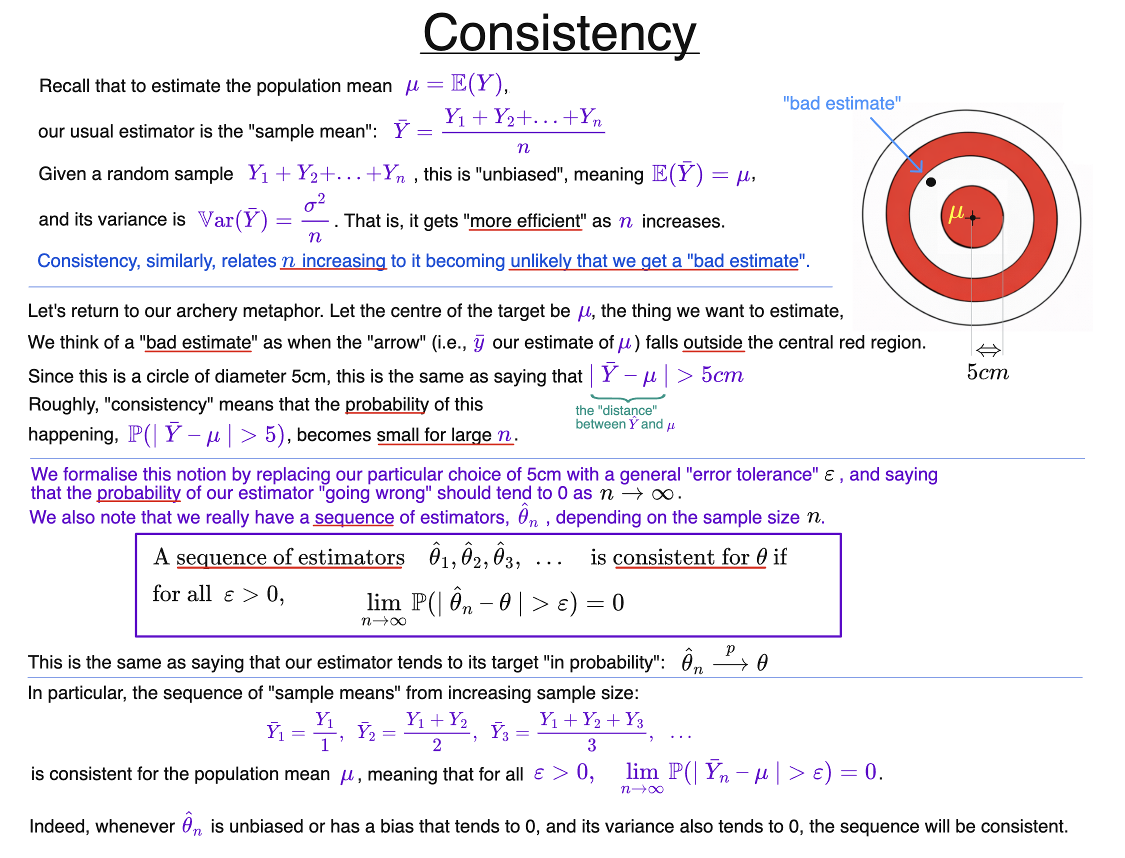
What Is a Consistent Estimator?

Suppose $\theta$ is an unknown quantity, and

$$\hat{\theta}_1,\hat{\theta}_2,\hat{\theta}_3,\dots$$

is a sequence of estimators, where $\hat{\theta}_n$ is the estimator we use when our sample size is $n$.

Roughly, the sequence is consistent for $\theta$ if the probability of getting an estimate that is “far away” from $\theta$ tends to $0$ as $n\to\infty$.

That is, having more data makes the possibility of our estimation “going wrong” increasingly unlikely.

Our next job is to formalise this intuition.

The Formal Definition

To make “far away” precise, first choose an error tolerance $\varepsilon>0$.

We say that our estimator has gone wrong by more than this tolerance when

$$|\hat{\theta}_n-\theta|>\varepsilon.$$

Consistency requires that, for every possible choice of $\varepsilon>0$, the probability of this event tends to $0$ as the sample size grows:

$$\forall\varepsilon>0,\qquad \lim_{n\to\infty}\mathbb{P}(|\hat{\theta}_n-\theta|>\varepsilon)=0.$$

The important point is that $\varepsilon$ can be arbitrarily small. Whatever value is chosen, as the sample size grows, our estimator becomes increasingly unlikely to lie outside this fixed distance $\varepsilon$ from the true value.

Example: The Sample Mean

Consider the sequence of sample means

$$\bar Y_1=\frac{Y_1}{1},\qquad \bar Y_2=\frac{Y_1+Y_2}{2},\qquad \bar Y_3=\frac{Y_1+Y_2+Y_3}{3},\qquad\dots$$

where $Y_1,Y_2,\dots$ form a random sample with population mean

$$\mu=\mathbb{E}(Y_i).$$

The sequence $\bar Y_n$ is consistent for $\mu$. That is,

$$\forall\varepsilon>0,\qquad \lim_{n\to\infty}\mathbb{P}(|\bar Y_n-\mu|>\varepsilon)=0.$$

This is precisely the weak law of large numbers.

A Useful Sufficient Condition

Recall that the bias of an estimator is

$$\operatorname{Bias}_{\theta}(\hat{\theta}_n)=\mathbb{E}(\hat{\theta}_n)-\theta.$$

A useful sufficient condition for consistency is that, as $n\to\infty$,

$$\operatorname{Bias}_{\theta}(\hat{\theta}_n)\to0$$

and

$$\operatorname{Var}(\hat{\theta}_n)\to0.$$

If both happen, the estimator becomes centred increasingly close to $\theta$, while also becoming increasingly concentrated around its own mean. Together, these are enough to guarantee consistency.

The converse is not true. A sequence can be consistent even if its bias or variance does not tend to $0$. Roughly, this happens if we have a sequence of estimators that are increasingly unlikely to “go wrong” as $n$ increases, yet when they do go wrong, they do so in an increasingly catastrophic way. That is, the errors an estimator makes on those increasingly rare occasions become correspondingly more extreme – meaning that the bias and/or variance do not vanish overall.

Consistency and Convergence in Probability

Consistency is exactly the statement that our sequence of estimators converges in probability to the constant $\theta$:

$$\hat{\theta}_n\overset{p}{\longrightarrow}\theta\qquad\text{as }n\to\infty.$$

So, consistency is not a new type of convergence. It is the name we give to convergence in probability when a sequence of estimators converges to the constant quantity it is intended to estimate.

Background

• Convergence in Probability

• Estimators as Random Variables

• Weak vs Strong Law of Large Numbers