What Is the Mean Squared Error (MSE)?

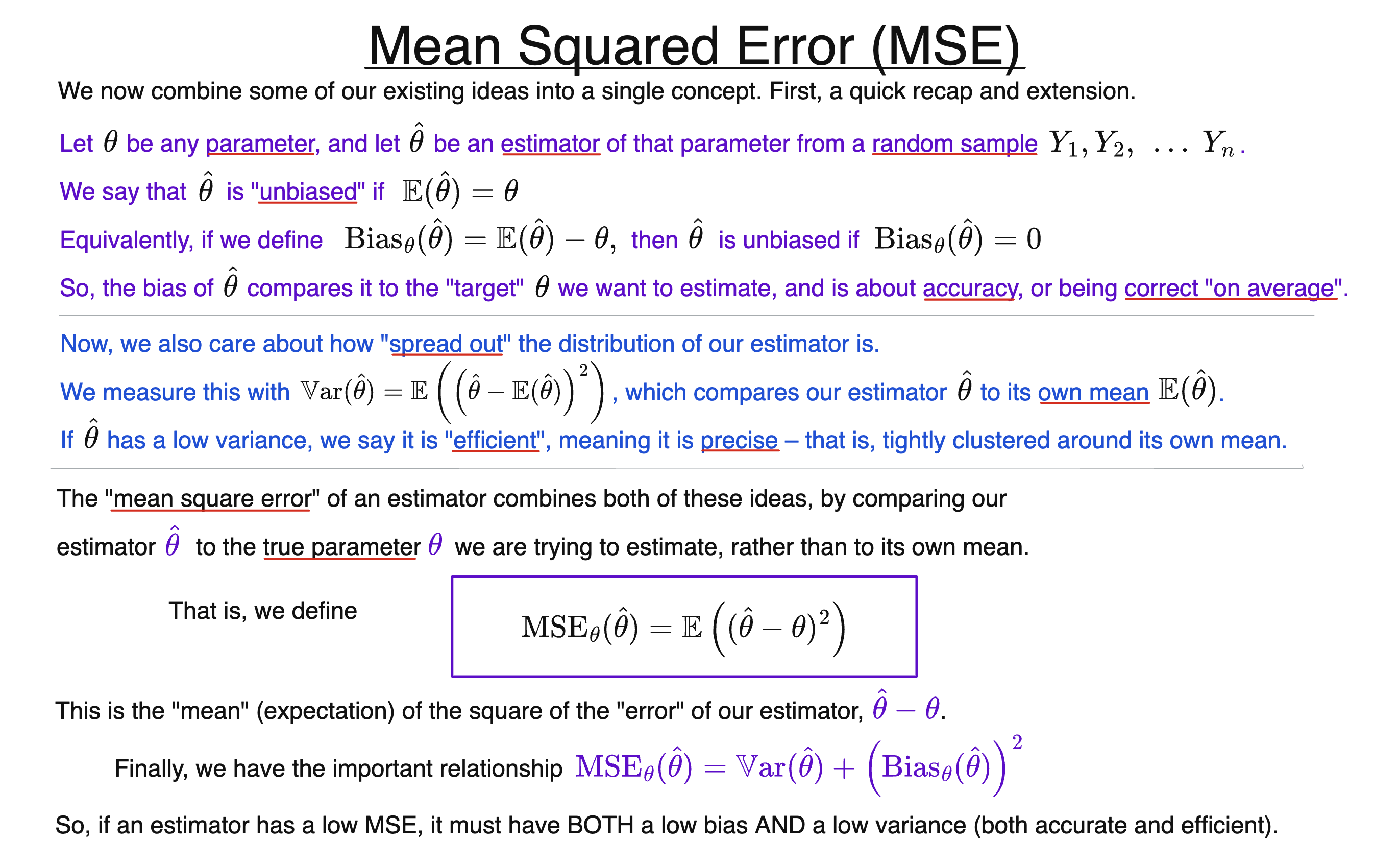
The mean squared error, or MSE, of an estimator $\hat{\theta}$ of a parameter $\theta$ is the expected squared difference between the estimator and the true value of the parameter:

$$\operatorname{MSE}_ {\theta}(\hat{\theta})=\mathbb{E}\left((\hat{\theta}-\theta)^2\right).$$

We can think of $\hat{\theta}-\theta$ as the error in our estimator. As usual, we square this error to prevent positive and negative deviations from “cancelling out” when we take an expectation.

Unlike variance, which measures how far an estimator tends to lie from its own mean, MSE measures how far it tends to lie from the true value $\theta$ we are trying to estimate.

This allows MSE to capture both accuracy and precision at once.

The Bias-Variance Decomposition

Recall that the bias of an estimator is

$$\operatorname{Bias}_ {\theta}(\hat{\theta})=\mathbb{E}(\hat{\theta})-\theta,$$

while its variance measures how spread out it is around its own expected value.

These two ideas come together in the important bias-variance decomposition:

$$\operatorname{MSE}_ {\theta}(\hat{\theta})=\operatorname{Var}(\hat{\theta})+\operatorname{Bias}_ {\theta}(\hat{\theta})^2.$$

The first term is the variance of $\hat{\theta}$, while the second is its squared bias.

Accuracy and Precision

The decomposition provides insight into what is required for a small MSE.

A small bias means that the estimator is accurate, or close to being “correct on average”. A small variance means that it is precise, with relatively little random variation from sample to sample.

Since both terms in

$$\operatorname{MSE}_ {\theta}(\hat{\theta})=\operatorname{Var}(\hat{\theta})+\left(\operatorname{Bias}_ {\theta}(\hat{\theta})\right)^2$$

are non-negative, a low MSE requires both a low variance and a low bias.

This also captures the bias-variance trade-off: sometimes accepting a little bias can substantially reduce variance, and thereby give us a lower MSE overall.

MSE and Consistency

MSE also gives us a useful sufficient condition for consistency.

Suppose we have a sequence of estimators

$$\hat{\theta}_1,\hat{\theta}_2,\dots$$

and

$$\operatorname{MSE}_ {\theta}(\hat{\theta}_n)\to0$$

as $n\to\infty$.

Then the sequence is consistent for $\theta$:

$$\hat{\theta}_n\overset{p}{\longrightarrow}\theta.$$

The converse is not true. As we saw when discussing consistency, an estimator can become increasingly unlikely to “go wrong”, while the errors on those increasingly rare occasions become increasingly extreme. It can therefore be consistent even though its MSE does not tend to $0$.

Background

• Expected Values

• Variance and Standard Deviation

• Estimators as Random Variables