The True Model

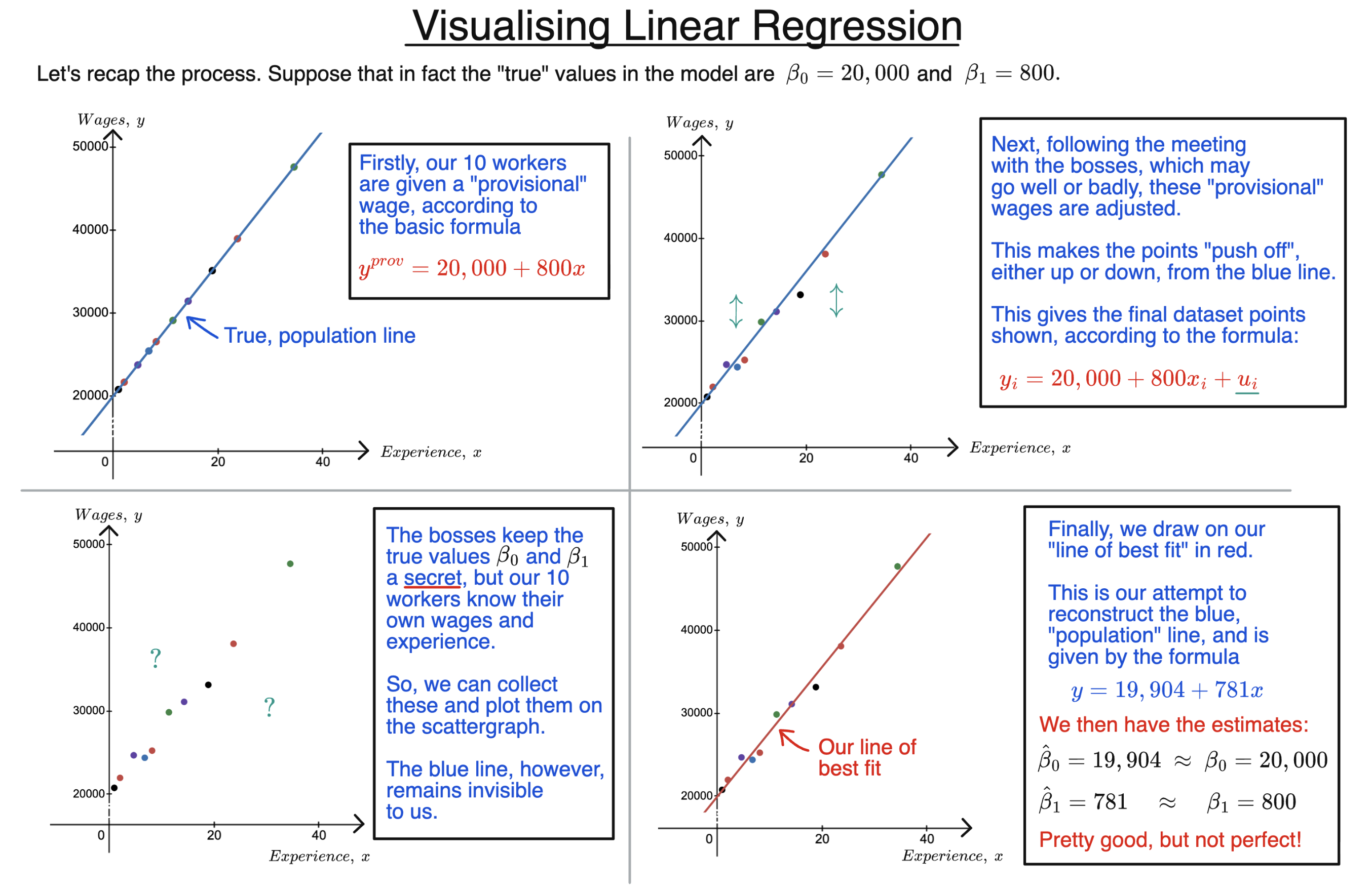
The graphs above give us a visual recap of our linear regression method.

Suppose that the true model is

$$Y=20{,}000+800X+U.$$

The coefficients are therefore $\beta_0=20{,}000$ and $\beta_1=800.$

If we temporarily ignore the error term, these coefficients give us the straight blue line in the first graph:

$$y=20{,}000+800x.$$

We can think of this as the true model line, representing the relationship in the model before the error term is applied. In our main example, we can think of this as a “provisional wage” before we see how much the bosses like the worker.

From the Model to the Data

Difficulties start to come in when the error term $U$ introduces variation around this line, pushing the points either “up” or “down” from it, as shown in the second graph.

For each individual, a positive value of the error term pushes the observed value of $Y$ above the initial model line, while a negative value pushes it below this line.

This gives us the scattered points shown in the second graph.

The issue is that, for a real regression, after collecting our data, we would see only these final, scattered points, as shown in graph 3. The true coefficients $\beta_0$ and $\beta_1$ are unknown, and hence the blue population line would remain invisible to us.

Estimating the Hidden Line

Linear regression attempts to reconstruct where this hidden line is, using only the data we have collected and plotted on the scatter diagram. Essentially, we just look at the line of best fit!

This line is drawn on in red in graph 4. Its equation is:

$$y=19{,}904+781x.$$

Comparing this directly to our model formula:

$$Y=\beta_0+\beta_1X+U.$$

We therefore estimate

$$\hat\beta_0=19{,}904$$

and

$$\hat\beta_1=781.$$

Unlike in a real regression, in the example in the slide, we are in the special position of actually knowing that the true values are $\beta_0=20{,}000$ and $\beta_1=800.$

So, we can see that our estimates are not exactly equal to these true values. However, they are fairly close!

Background

• Estimands, Estimates, and Estimators
• Linear Models
• Working with Data