Different Samples, Different Estimates

We have now settled the question of how to choose a line of best fit: using OLS, we select the intercept and slope that minimise the sum of squared residuals.

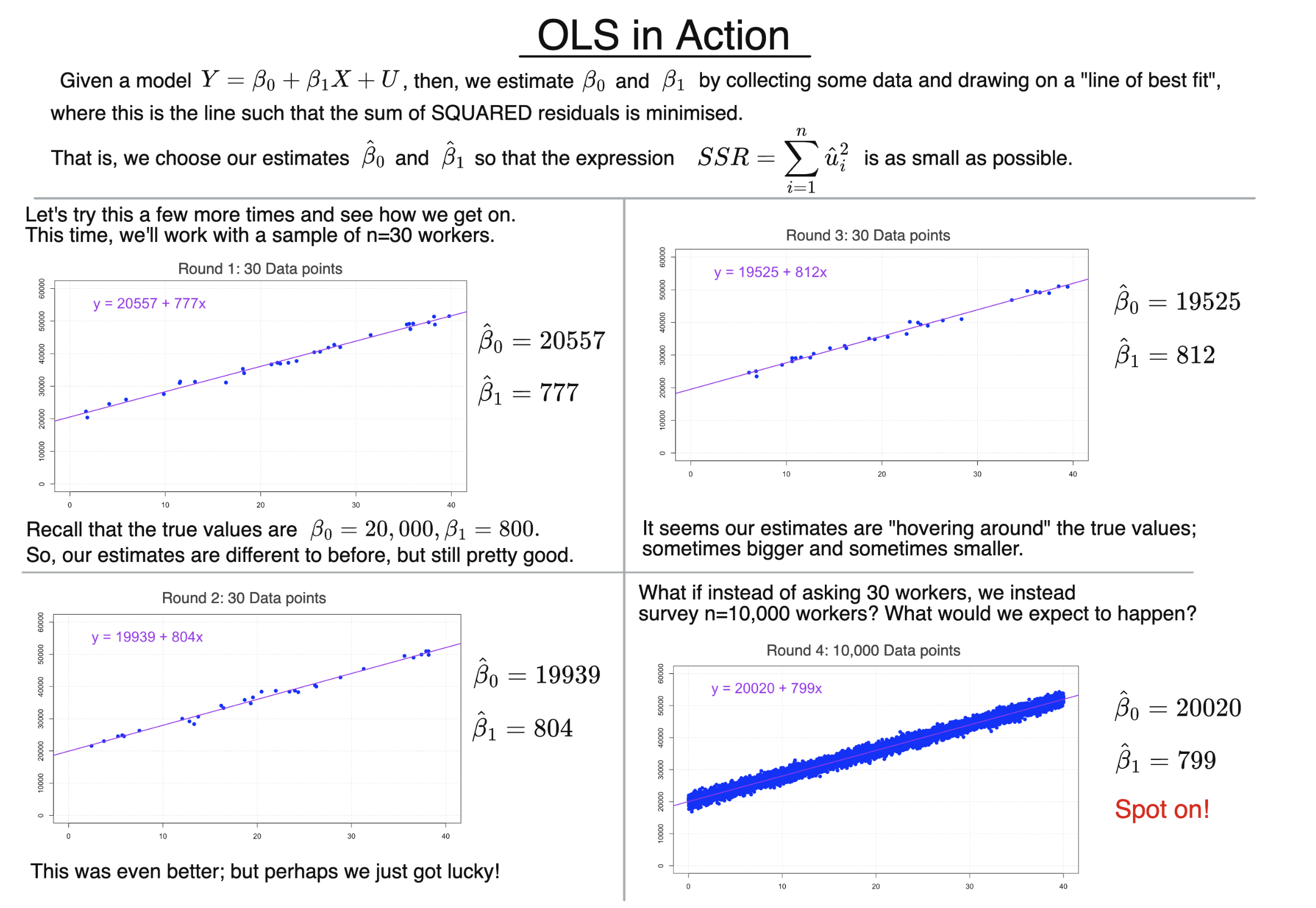
The slide above shows the process in action several times.

We return to our main example, continuing to assume that the true model is

$$Y=20{,}000+800X+U.$$

So, the true coefficients are $\beta_0=20{,}000$ and $\beta_1=800.$

Of course, this is just for illustration; ordinarily we wouldn’t know the true values – if we did, we wouldn’t need to run a regression at all, and could go and do something else instead!

The slide begins with three different samples of $30$ workers. Each time, we run exactly the same OLS procedure. Yet each sample gives us slightly different estimates of $\beta_0$ and $\beta_1.$

Why the Estimates Change

For the three samples, our slope estimates are

$$\hat\beta_1=777,\qquad 804,\qquad 812.$$

Overall, the slope estimates seem to be “hovering around” the true value – sometimes a little too high, and sometimes a little too low. None is exactly equal to the true value $\beta_1=800$, although all three are reasonably close. The same thing happens with the intercept.

Even though the underlying model stays exactly the same, and we use exactly the same method, the particular data we happen to collect will vary from one sample to another – and as a result, our OLS estimates vary too.

In a real regression study, we’d usually only run the regression once, rather than collecting several different samples – and we wouldn’t know the true values to compare our estimates with. So, we have to hope that our estimates come out close to the truth!

There is some luck involved here – though it is also possible to evaluate the reliability of our method mathematically, and sometimes improve on it.

What Happens with More Data?

The final graph repeats the exercise with a much larger sample, now consisting of $10{,}000$ randomly chosen workers.

This time, we obtain

$$\hat\beta_0=20{,}020$$

and

$$\hat\beta_1=799.$$

These are extremely close to the true values $20{,}000$ and $800.$

This suggests an encouraging idea: with more data, our OLS estimates may become more accurate.

These examples give us some useful intuition. But to say something more rigorous about how well OLS performs, and whether it is a reliable method, we need to return to the tools supplied by probability and statistics.

Background

• Random Samples
• Estimators as Random Variables
• OLS Estimation