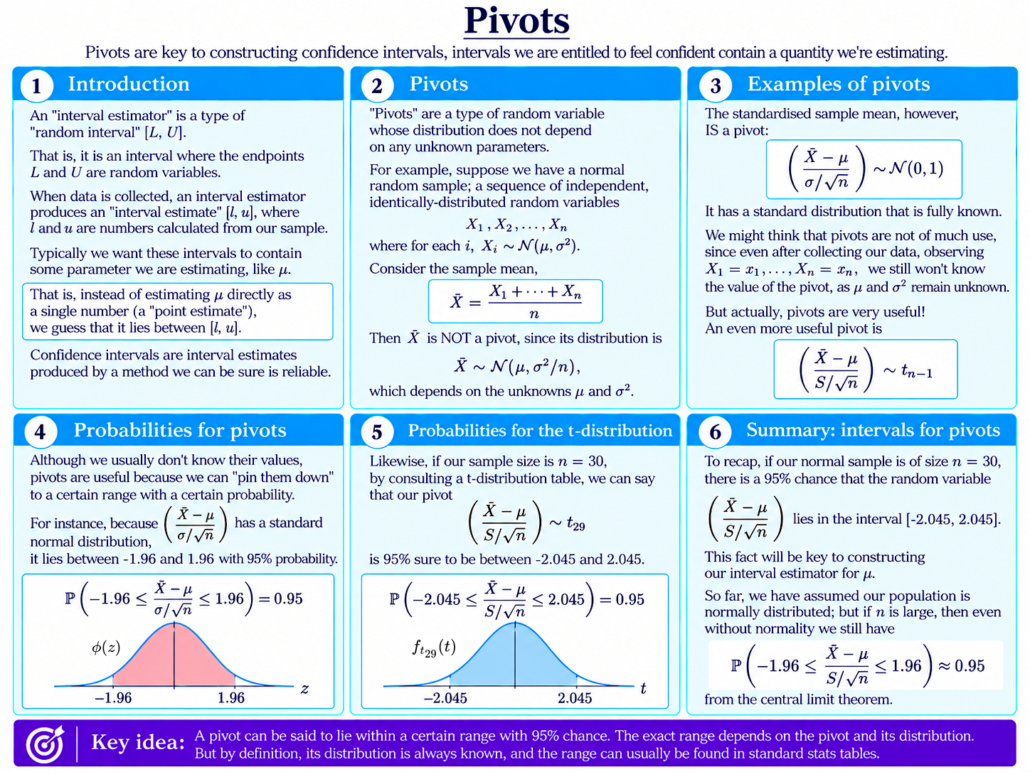
What Is a Pivot?

So far, most of our estimators have produced a single numerical guess of an unknown quantity.

A confidence interval instead gives us a whole interval of plausible values.

Before collecting the data, we can think of the method that produces this as an interval estimator:

$$[L,U],$$

where the endpoints $L$ and $U$ are themselves random variables.

After collecting our data, these become particular numbers $l$ and $u$, giving the interval estimate

$$[l,u].$$

Confidence intervals are a particular kind of interval estimate. To begin to understand how they are constructed, we must define an important new concept: a pivot.

A pivot is a random variable whose probability distribution is fully known – that is, does not depend on any unknown parameters.

An Example

Suppose

$$X_1,X_2,\dots,X_n$$

form a normal random sample, with

$$X_i\sim\mathcal{N}(\mu,\sigma^2).$$

Consider the sample mean

$$\bar X=\frac{X_1+X_2+\dots+X_n}{n}.$$

Although we know that

$$\bar X\sim\mathcal{N}\left(\mu,\frac{\sigma^2}{n}\right),$$

$\bar X$ is not a pivot. Its distribution still depends on the unknown quantities $\mu$ and $\sigma^2$.

But if we standardise it,

$$\frac{\bar X-\mu}{\sigma/\sqrt{n}}\sim\mathcal{N}(0,1),$$

we obtain a pivot.

The expression itself still contains the unknown parameters $\mu$ and $\sigma$. But its distribution no longer does: it is exactly a standard normal distribution.

Why Are Pivots Useful?

At first this might seem slightly odd. Even after collecting our data, we usually cannot calculate the numerical value of the pivot above because $\mu$ and $\sigma$ are unknown. That is, this pivot is not a “statistic”.

However, although it is unobservable, we do know how a pivot behaves.

For instance, a standard normal random variable lies between $-1.96$ and $1.96$ with probability $0.95$. Therefore,

$$\mathbb{P}\left(-1.96\leq\frac{\bar X-\mu}{\sigma/\sqrt{n}}\leq1.96\right)=0.95.$$

So, although we cannot work out its value from our data alone, we can still “pin it down” to a particular range with a known probability.

This is exactly the sort of probability statement we will use to construct confidence intervals.

When $\sigma$ Is Unknown

Usually, of course, the population standard deviation $\sigma$ is itself unknown.

For a normal random sample, replacing $\sigma$ with the sample standard deviation $S$ gives another pivot:

$$\frac{\bar X-\mu}{S/\sqrt{n}}\sim t_{n-1}.$$

Its distribution is now a $t$-distribution with $n-1$ degrees of freedom. Crucially, although it depends on $n$, this is just the size of our sample, and therefore know to us – so, its distribution is fully known.

For example, if $n=30$,

$$\frac{\bar X-\mu}{S/\sqrt{30}}\sim t_{29}.$$

From the t-distribution, we can find that

$$\mathbb{P}\left(-2.045\leq\frac{\bar X-\mu}{S/\sqrt{30}}\leq2.045\right)=0.95.$$

Again, we have trapped an unknown pivot inside a known interval with 95% probability.

That is the key ingredient we need for constructing a confidence interval.

For Large Samples

The same basic idea also survives beyond normally distributed populations.

For large $n$, the Central Limit Theorem allows us to use the “approximate pivot”:

$$\frac{\bar X-\mu}{S/\sqrt{n}}\approx\mathcal{N}(0,1),$$

giving approximately

$$\mathbb{P}\left(-1.96\leq\frac{\bar X-\mu}{S/\sqrt{n}}\leq1.96\right)\approx0.95.$$

Background

• $t$-Distribution

• Central Limit Theorem