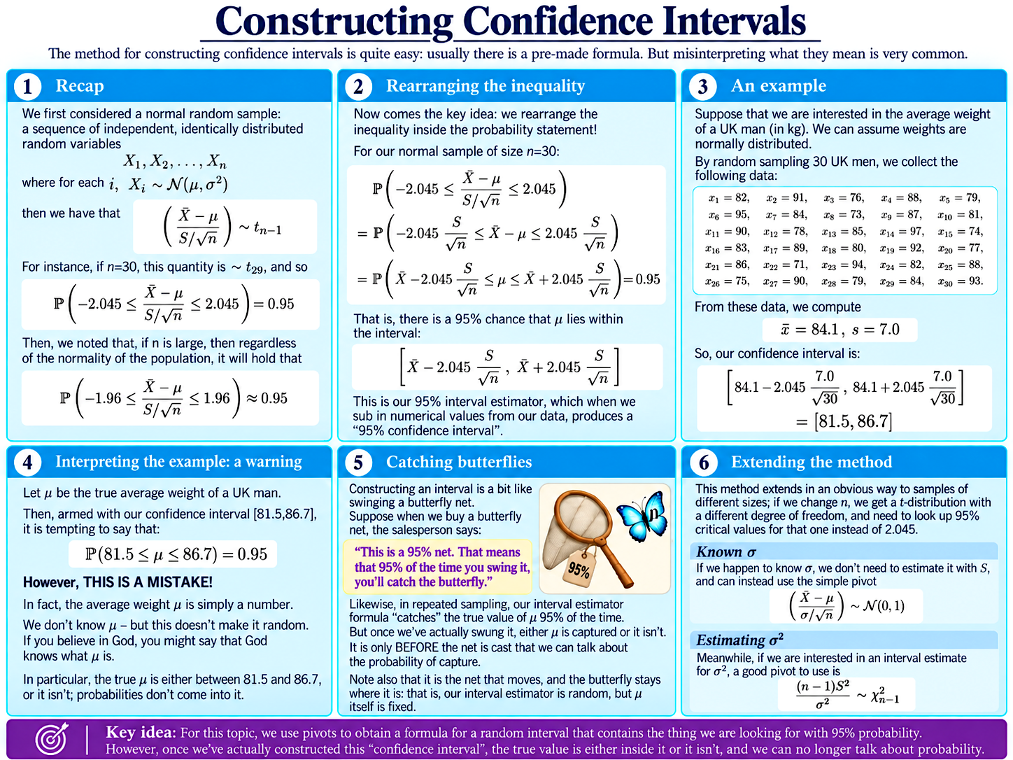
Constructing a Confidence Interval

Recall that if

$$X_1,X_2,\dots,X_n$$

form a normal random sample, then

$$\frac{\bar X-\mu}{S/\sqrt{n}}\sim t_{n-1}.$$

This gives us a “pivot” – a random variable whose distribution is completely known, even though the population mean $\mu$ and variance $\sigma^2$ are unknown.

Suppose, for example, that $n=30$. The middle 95% of a $t_{29}$ distribution lies between approximately $-2.045$ and $2.045$. Hence,

$$\mathbb{P}\left(-2.045\leq\frac{\bar X-\mu}{S/\sqrt{30}}\leq2.045\right)=0.95.$$

Now comes the key step: we rearrange the inequalities inside the probability statement to make $\mu$ the subject.

This gives

$$\mathbb{P}\left(\bar X-2.045\frac{S}{\sqrt{30}}\leq\mu\leq\bar X+2.045\frac{S}{\sqrt{30}}\right)=0.95.$$

So the random interval

$$\left[\bar X-2.045\frac{S}{\sqrt{30}},\ \bar X+2.045\frac{S}{\sqrt{30}}\right]$$

contains the true population mean $\mu$ with probability $0.95$.

This is our 95% confidence interval estimator.

A Numerical Example

Suppose we randomly sample $30$ UK men and record their weights.

For the data on the slide, we obtain

$$\bar x=84.1,\qquad s=7.0.$$

Substituting these observed values into our interval estimator gives

$$\left[84.1-2.045\frac{7.0}{\sqrt{30}},\ 84.1+2.045\frac{7.0}{\sqrt{30}}\right].$$

Hence, our 95% confidence interval is approximately

$$[81.5,\ 86.7].$$

This is now an ordinary numerical interval rather than a random one.

What Does “95% Confidence” Mean?

This is where confidence intervals are very commonly misinterpreted.

Once we have obtained the particular interval

$$[81.5,\ 86.7],$$

it is tempting to write

$$\mathbb{P}(81.5\leq\mu\leq86.7)=0.95.$$

But in our framework, this is not correct.

The true population mean $\mu$ is a fixed number. We do not know what it is, but our ignorance does not make it random. Either $\mu$ lies between $81.5$ and $86.7$, or it does not.

The probability statement applies before we collect the data, when the endpoints of our interval are still random variables:

$$\mathbb{P}\left(\bar X-2.045\frac{S}{\sqrt{30}}\leq\mu\leq\bar X+2.045\frac{S}{\sqrt{30}}\right)=0.95.$$

In repeated sampling, this method will produce intervals containing the true value $\mu$ 95% of the time.

Once we have collected our particular sample, the interval has already either captured $\mu$ or missed it.

Catching Butterflies

A useful way to picture this is to imagine trying to catch a butterfly with a net.

The butterfly represents the fixed population mean $\mu$. It stays exactly where it is.

The confidence interval is the net. Before we collect our data, we do not know exactly where the net will land: its position depends on the random sample we happen to obtain.

A 95% confidence interval method is like a net which catches the butterfly on 95% of our swings.

Once we have actually swung the net, though, the butterfly is either inside it or outside it. There is no longer a 95% probability attached to that particular event.

The important point is that the net moves; the butterfly does not – and after each swing, we have either a success or a failure.

Of course, the analogy breaks down in one way: after constructing a confidence interval, we are unable to tell whether we have “captured” the true $\mu$ or not. This is because we don’t know $\mu$. If we did, we could give up with the confidence intervals altogether, and do something else instead – like underwater basket weaving!

Explore the Confidence Interval

For a normal population with unknown variance, a confidence interval for $\mu$ has the general form

$$ \left[ \bar{x}-t^* \frac{s}{ \sqrt{n}}, \ \bar{x} + t^* \frac{s}{\sqrt{n}} \right],$$

where $t^* $ is chosen from the $t$-distribution with $n-1$ degrees of freedom, according to the confidence level we want. That is, if $T\sim t_{n-1}$, then $t^* $ is a value such that $\mathbb{P}(-t^* <T<t^* )$ is equal to the desired confidence level. $t^* $ can be found with standard stats tables or software.

The interactive graph below lets you experiment with the observed sample mean $x_{mean}=\bar{x}$, the sample size $n$, the sample standard deviation $s$, and the percentage confidence level $P$.

Try changing each one separately and watch what happens to the interval.

Changing $\bar x$ moves the centre of the interval. Increasing $s$ makes it wider as there is more uncertainty. Increasing $n$ makes it narrower, as we have more information about $\mu$. Asking for a higher level of confidence also makes the interval wider: to be more confident of catching the butterfly, we need a bigger net!

You can move the sliders, or manually type in any value you like.

Some Extensions

The particular formula above assumed normally distributed data and an unknown population variance.

If $\sigma$ were known, we could instead use the standard normal pivot

$$\frac{\bar X-\mu}{\sigma/\sqrt n}\sim\mathcal{N}(0,1).$$

For large samples from non-normal populations, the Central Limit Theorem also allows us to construct approximately valid confidence intervals using the normal distribution.

We can also construct confidence intervals for quantities other than the population mean. For example, with normally distributed data, the chi-squared pivot

$$\frac{(n-1)S^2}{\sigma^2}\sim\chi^2_{n-1}$$

can be used to construct a confidence interval for the population variance $\sigma^2$.