What Is the t-Distribution?

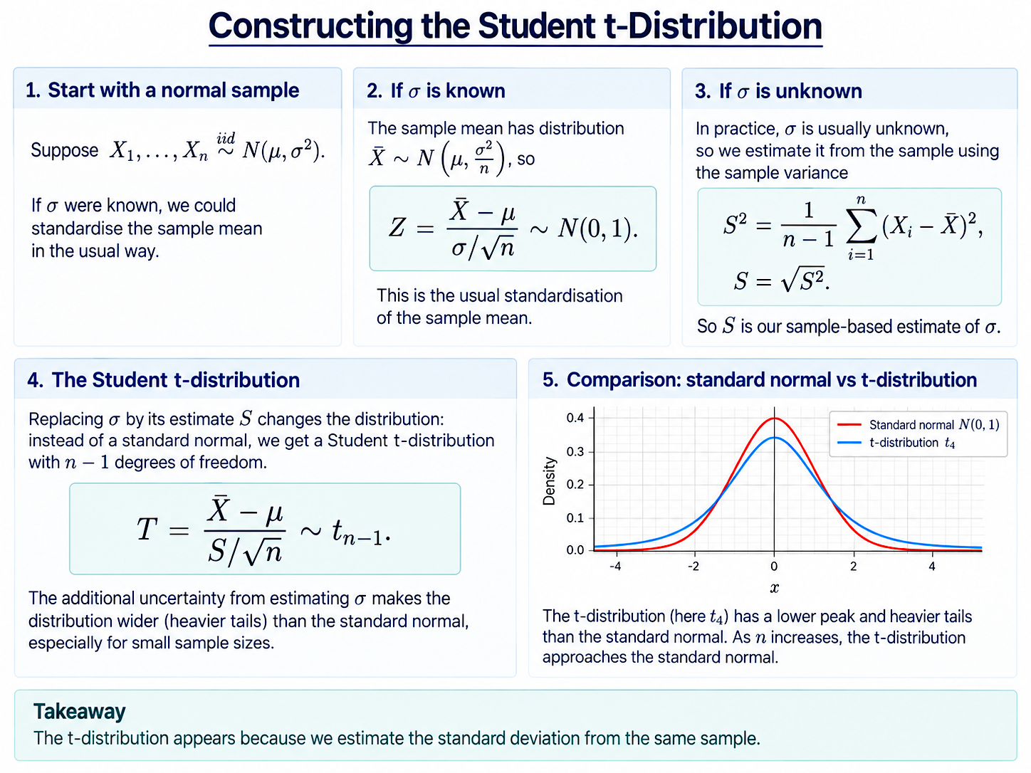
The Student t-distribution appears naturally when we standardise a sample mean, but have to estimate the population standard deviation from the same sample.

Suppose

$$X_1,\ldots,X_n \ \overset{\mathrm{iid}}{\sim}\mathcal{N}(\mu,\sigma^2).$$

Then the sample mean has distribution

$$\bar{X}\sim\mathcal{N}\left(\mu,\frac{\sigma^2}{n}\right).$$

If the population standard deviation $\sigma$ were known, we could standardise $\bar{X}$ in the usual way:

$$Z=\frac{\bar{X}-\mu}{\sigma/\sqrt{n}}\sim\mathcal{N}(0,1).$$

In practice, however, $\sigma$ is usually unknown.

We therefore resort to estimating it from the sample.

Replacing $\sigma$ with the Sample Standard Deviation

The sample variance is

$$S^2=\frac{1}{n-1}\sum_{i=1}^n(X_i-\bar{X})^2,$$

and the sample standard deviation is

$$S=\sqrt{S^2}.$$

Instead of dividing by the unknown quantity $\sigma/\sqrt{n}$, we divide by its sample-based estimate $S/\sqrt{n}$.

This gives

$$T=\frac{\bar{X}-\mu}{S/\sqrt{n}}.$$

This is where the t-distribution comes in. For a normally distributed random sample,

$$T\sim t_{n-1}.$$

That is, $T$ has a Student t-distribution with $n-1$ degrees of freedom.

This is the main practical reason the t-distribution is so important: it appears when we standardise using an estimated standard deviation rather than the true population standard deviation.

Why Is It Different from the Standard Normal?

If $\sigma$ were known, the denominator

$$\frac{\sigma}{\sqrt{n}}$$

would be fixed.

When we replace $\sigma$ with $S$, the denominator becomes random because $S$ depends on the particular sample we draw.

This makes extreme values more likely than under a standard normal distribution, giving the t-distribution its heavier tails.

Both distributions are symmetric around zero, but the t-distribution has a lower peak and heavier tails, particularly when the number of degrees of freedom is small.

Degrees of Freedom

When the t-distribution arises from a normal sample of size $n$ in this way, it has

$$n-1$$

degrees of freedom.

We write

$$T\sim t_{n-1}.$$

The number of degrees of freedom determines the shape of the distribution.

With only a few degrees of freedom, estimating $\sigma$ introduces noticeable additional uncertainty.

If $n$ is large, however, the sample standard deviation $S$ is likely to be a very accurate estimate of $\sigma$. It then matters much less that we use the estimate $S$ rather than the true value $\sigma$.

This is why the t-distribution becomes increasingly similar to the standard normal distribution as the number of degrees of freedom grows.

Interactive t-Distribution

The graph below lets you explore how the Student t-distribution changes with its degrees of freedom.

The thick red curve is the pdf of the t-distribution. The thin purple curve is the standard normal pdf, included for comparison.

Use the slider for $n$ to change the number of degrees of freedom. You can also choose values $c$ and $d$; the shaded region shows

$$\mathbb{P}(c\leq T\leq d).$$

For small values of $n$, the red t-distribution has visibly heavier tails than the standard normal.

As you increase $n$, the red pdf approaches the thin purple standard normal pdf. For sufficiently large values of $n$, the two are almost indistinguishable.

Why Is the t-Distribution Important?

The t-distribution is fundamental whenever we want to learn about an unknown population mean but do not know the population variance.

For normally distributed data, it allows us to account exactly for the additional uncertainty introduced by estimating $\sigma$ from the sample.

This makes it central to confidence intervals and hypothesis tests involving sample means.

The same basic idea appears repeatedly in econometrics. We often standardise an estimator by dividing by an estimated standard deviation rather than one that is known in advance.

The next page shows how the t-distribution can also be constructed mathematically from a standard normal random variable and an independent chi-squared random variable.

Background:

• Normal Distribution

• Variance and Standard Deviation

• Chi-Squared Distribution

• Estimating the Variance