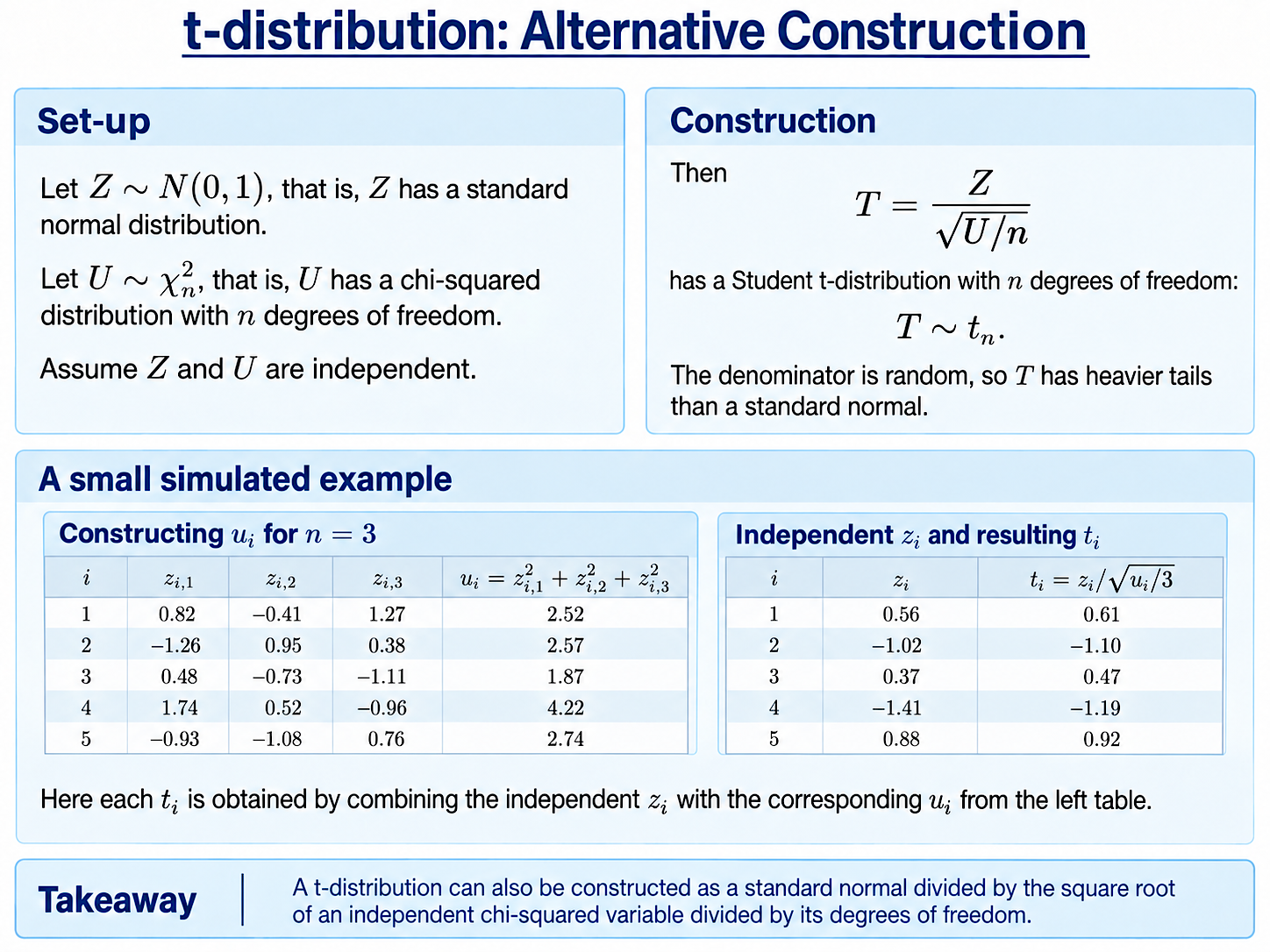
Another Way to Think About the t-Distribution

On the previous page, we saw that the t-distribution appears when we standardise a sample mean using an estimated standard deviation:

$$T=\frac{\bar{X}-\mu}{S/\sqrt{n}}.$$

There are already some clues here about what the t-distribution is made from.

The standardised sample mean on the top is normally distributed. Meanwhile, the estimated variance in the denominator is constructed from squared deviations from the sample mean, making it look rather like the chi-squared distributions we met earlier.

There is also a surprising fact hiding in the background. When the original sample is normally distributed, $\bar{X}$ and $S^2$ are independent random variables, even though both are calculated from the same sample.

This is suggestive of another, much cleaner way to construct the t-distribution directly.

Constructing a t-Distribution

Let

$$Z\sim\mathcal{N}(0,1)$$

and

$$U\sim\chi_n^2,$$

and assume that $Z$ and $U$ are independent.

Then construct

$$T=\frac{Z}{\sqrt{U/n}}.$$

The resulting random variable has a Student t-distribution with $n$ degrees of freedom:

$$T\sim t_n.$$

So the recipe is simple: take a standard normal random variable and divide it by the square root of an independent chi-squared random variable, divided by its degrees of freedom.

Why Does the t-Distribution Have Heavier Tails?

The numerator $Z$ has a standard normal distribution.

The important difference is the denominator:

$$\sqrt{\frac{U}{n}}.$$

This is itself random. Sometimes, by chance, it will take a very small value, making the resulting value of $T$ unusually large in magnitude.

Extreme values are therefore more likely than for a standard normal random variable, giving the t-distribution its characteristic heavier tails.

What Happens as the Degrees of Freedom Increase?

This construction also explains why the t-distribution approaches the standard normal as $n$ grows.

For

$$U\sim\chi_n^2,$$

we have the standard result that

$$\mathbb{E}(U)=n$$

and

$$\operatorname{Var}(U)=2n.$$

Dividing by $n$ gives

$$\mathbb{E}\left(\frac{U}{n}\right)=1$$

and

$$\operatorname{Var}\left(\frac{U}{n}\right)=\frac{2}{n}.$$

So $U/n$ always has expected value $1$, while its variance becomes smaller and smaller as $n$ increases.

For large $n$, $U/n$ is therefore very likely to lie close to $1$. The denominator

$$\sqrt{\frac{U}{n}}$$

also becomes increasingly concentrated around $1$: its expected value approaches $1$ and its variance approaches $0$.

Our construction

$$T=\frac{Z}{\sqrt{U/n}}$$

then becomes increasingly similar to simply

$$Z.$$

This gives a direct explanation for why the t-distribution approaches the standard normal distribution as its degrees of freedom increase.

Interactive t-Distribution

The graph below shows this change in the pdf.

The thick red curve is the pdf of the t-distribution. The thin purple curve is the standard normal pdf, included for comparison.

Use the slider for $n$ to change the number of degrees of freedom. You can also choose values $c$ and $d$; the shaded region shows

$$\mathbb{P}(c\leq T\leq d).$$

For small values of $n$, the heavier tails of the t-distribution are clearly visible.

As $n$ increases, $U/n$ becomes more tightly concentrated around $1$. The random denominator therefore has less and less effect, and the thick red t-distribution pdf approaches the thin purple standard normal pdf.

Summary: Two Views of the t-Distribution

We now have two useful ways to think about the Student t-distribution.

In applications, it appears naturally when a standard deviation must be estimated from the sample rather than known in advance.

Mathematically, it can be constructed from two familiar distributions:

$$T=\frac{Z}{\sqrt{U/n}},$$

where $Z\sim\mathcal{N}(0,1)$, $U\sim\chi_n^2$, and $Z$ and $U$ are independent.

These are two different ways of seeing the same distribution.

Background:

• t-Distribution

• Chi-Squared Distribution

• Normal Distribution