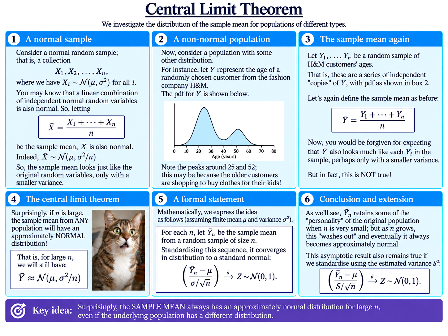
What Is the Central Limit Theorem?

Suppose

$$Y_1,Y_2,\dots,Y_n$$

form a random sample from a population, with common mean

$$\mu=\mathbb{E}(Y_i)$$

and variance

$$\sigma^2=\operatorname{Var}(Y_i).$$

As usual, let

$$\bar Y_n=\frac{Y_1+Y_2+\dots+Y_n}{n}$$

be the sample mean.

If the original population is normally distributed, the distribution of $\bar Y_n$ follows quite naturally. A linear combination of independent normal random variables is itself normal, so

$$Y_i\sim\mathcal{N}(\mu,\sigma^2)\quad\Longrightarrow\quad\bar Y_n\sim\mathcal{N}\left(\mu,\frac{\sigma^2}{n}\right).$$

Now for the surprising part.

Suppose instead that the original population is not normal at all. It might be skewed, lumpy, or have several peaks. You might reasonably expect the sample mean to retain the same sort of shape as the sample size grows, perhaps just getting thinner as its variance reduces.

But this is not what happens at all!

In fact, as the sample size becomes large, the distribution of the sample mean always becomes approximately normal:

$$\bar Y_n\approx\mathcal{N}\left(\mu,\frac{\sigma^2}{n}\right).$$

This remarkable fact is the Central Limit Theorem.

For smaller samples, the distribution of $\bar Y_n$ may retain some of the “personality” of the original population. As $n$ grows, however, this is increasingly “washed out”, and the familiar bell-shaped normal distribution emerges.

Note in particular that the original population does not become normal as the sample size increases. Sampling does not change the population at all! It is only our sample mean that becomes approximately normally distributed.

There is no single sample size at which this suddenly happens; how quickly the approximation becomes convincing depends partly on the shape of the original population, as we explore on the next page.

The Formal Central Limit Theorem

There is a slight complication in stating the theorem formally.

As $n$ changes, the approximate distribution

$$\mathcal{N}\left(\mu,\frac{\sigma^2}{n}\right)$$

changes too. So we cannot simply say that $\bar Y_n$ converges in distribution to this changing normal distribution.

Instead, we standardise the sample mean:

$$\frac{\bar Y_n-\mu}{\sigma/\sqrt{n}}.$$

Now, mathematically, for an IID sequence with finite mean $\mu$ and finite variance $\sigma^2$, the Central Limit Theorem states that

$$\frac{\bar Y_n-\mu}{\sigma/\sqrt{n}}\overset{d}{\longrightarrow}Z,$$

where

$$Z\sim\mathcal{N}(0,1).$$

That is, the distribution of the standardised sample mean becomes increasingly close to the standard normal distribution as $n\to\infty$.

We therefore say that the sample mean is asymptotically normal.

What If We Don’t Know $\sigma$?

The expression above contains the population standard deviation $\sigma$, which we usually do not know.

But we already have a natural estimator for it: the sample standard deviation. Recall that

$$S_n=\sqrt{S_n^2}=\sqrt{\frac{(Y_1-\bar Y_n)^2+(Y_2-\bar Y_n)^2+\dots+(Y_n-\bar Y_n)^2}{n-1}}.$$

Fortunately, we can replace $\sigma$ with $S_n$, and the same limiting result still holds:

$$\frac{\bar Y_n-\mu}{S_n/\sqrt{n}}\overset{d}{\longrightarrow}Z,$$

where

$$Z\sim\mathcal{N}(0,1).$$

The intuition is straightforward. As the sample size grows, $S_n$ becomes increasingly close to the true value $\sigma$, so replacing $\sigma$ with $S_n$ matters less and less.

In fact, this result is more general: we could replace $\sigma$ with any consistent estimator of it, and the same limiting distribution would remain.

• Convergence in Distribution