Why Standardise a Normal Random Variable?
Suppose
$$X\sim\mathcal{N}(\mu,\sigma^2).$$
Different values of $\mu$ and $\sigma$ give us different normal distributions.
If we wanted to find probabilities using statistical tables, it would not be practical to have a separate table for every possible combination of $\mu$ and $\sigma$.
Instead, we can standardise $X$. This transforms it into a standard normal random variable
$$Z\sim\mathcal{N}(0,1).$$
To standardise $X$, we subtract its mean and divide by its standard deviation:
$$Z=\frac{X-\mu}{\sigma}.$$
This works as follows. Firstly, we have
$$\mathbb{E}(X-\mu)=\mathbb{E}(X)-\mu=\mu-\mu=0.$$
So, subtracting $\mu$ from $X$ changes its mean from $\mu$ to $0$.
Likewise, dividing by $\sigma$ then makes its variance equal to $1$:
$$\operatorname{Var}\left(\frac{X-\mu}{\sigma}\right)=\frac{\operatorname{Var}(X-\mu)}{\sigma^2}=\frac{\operatorname{Var}(X)}{\sigma^2}=\frac{\sigma^2}{\sigma^2}=1.$$
Here we remember that when a constant is taken outside the variance, it is squared. By contrast, adding or subtracting a constant has no effect on the spread.
Any normally distributed random variable can be converted into the standard normal distribution in this way.
Standardising Probabilities
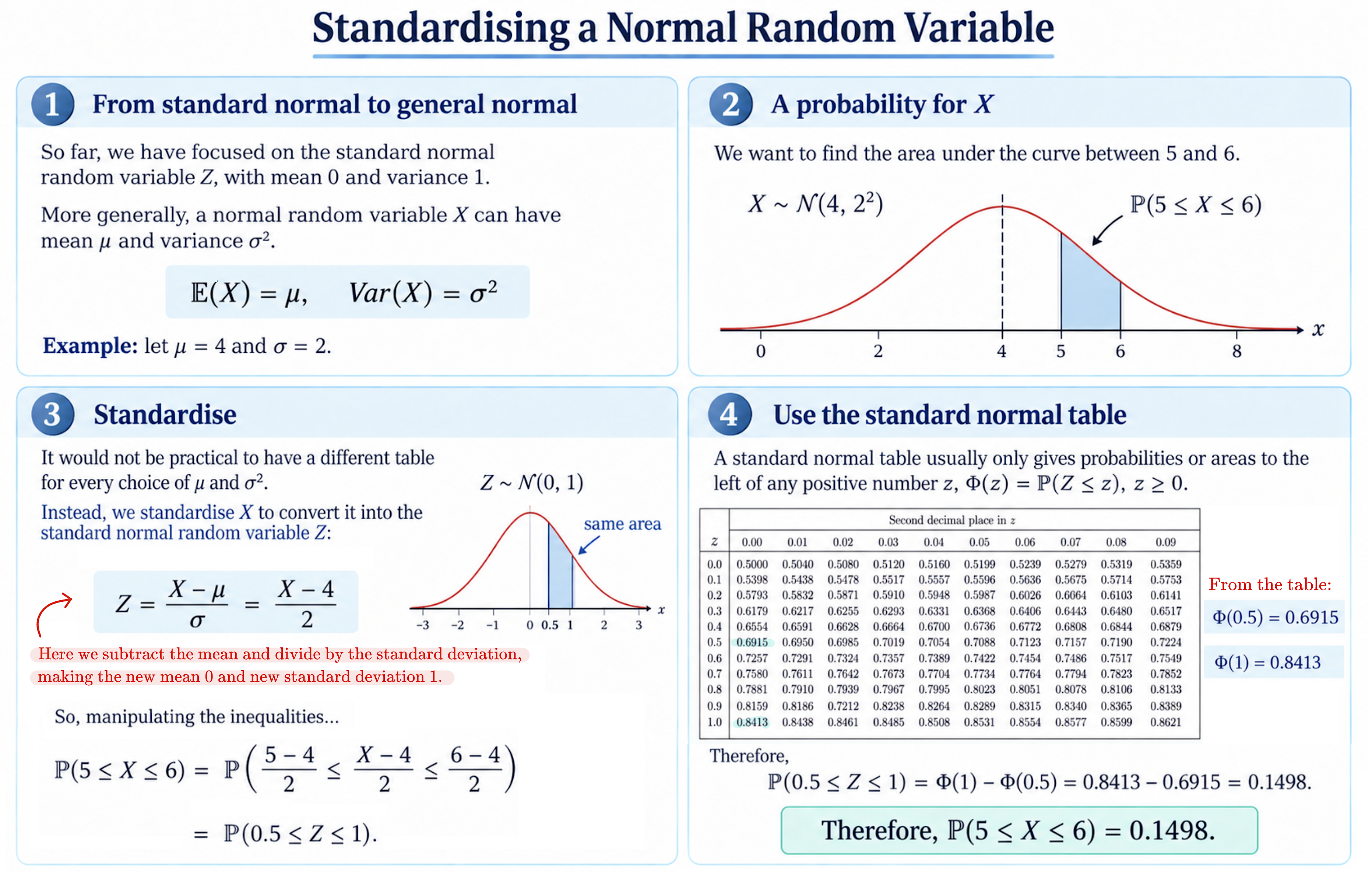
Standardisation is particularly useful when we want to find probabilities.
Suppose
$$X\sim\mathcal{N}(4,2^2),$$
and we want to calculate
$$\mathbb{P}(5\leq X\leq6).$$
Here,
$$\mu=4$$
and
$$\sigma=2.$$
We recall that we can add or subtract the same quantity from both sides of an inequality. We can also multiply or divide each side by any positive number. So, we may standardise all three terms in our inequality by subtracting $4$ and dividing by $2$:
$$\mathbb{P}(5\leq X\leq6)=\mathbb{P}\left(\frac{5-4}{2}\leq\frac{X-4}{2}\leq\frac{6-4}{2}\right).$$
Since
$$Z=\frac{X-4}{2},$$
this becomes
$$\mathbb{P}(5\leq X\leq6)=\mathbb{P}(0.5\leq Z\leq1).$$
We have therefore converted a probability involving $X\sim\mathcal{N}(4,2^2)$ into an equivalent probability involving the standard normal random variable $Z$.
This is convenient, because we can now find the probability from a standard table. Alternatively, you can use the applet below.
More generally, if $X\sim\mathcal{N}(\mu,\sigma^2)$, then
$$\mathbb{P}(c\leq X\leq d)=\mathbb{P}\left(\frac{c-\mu}{\sigma}\leq Z\leq\frac{d-\mu}{\sigma}\right).$$
Using the Standard Normal Table
A common type of standard normal table gives the cdf
$$\Phi(z)=\mathbb{P}(Z\leq z).$$
In our example, the table gives
$$\Phi(0.5)=0.6915$$
and
$$\Phi(1)=0.8413.$$
These are both probabilities to the left of the corresponding values.
To find the probability between $0.5$ and $1$, we therefore subtract the smaller area from the larger one:
$$\mathbb{P}(0.5\leq Z\leq1)=\Phi(1)-\Phi(0.5).$$
Hence,
$$\mathbb{P}(0.5\leq Z\leq1)=0.8413-0.6915=0.1498.$$
Since standardising did not change the event whose probability we wanted to find,
$$\mathbb{P}(5\leq X\leq6)=0.1498.$$
So the overall procedure is:
-
Standardise the values using $z=(x-\mu)/\sigma$.
-
Rewrite the probability in terms of the standard normal random variable $Z$.
-
Use the standard normal table or the applet below to find the required area.
Explore the Standard Normal Distribution
The interactive graph below works with the standard normal distribution only, so
$$Z\sim\mathcal{N}(0,1).$$
You can choose two values, $c$ and $d$, to calculate
$$\mathbb{P}(c\leq Z\leq d).$$
The shaded region shows this probability as an area under the standard normal pdf.
The horizontal axis shows possible values of $z$, and the graph highlights the interval from $c$ to $d$.
This applet is useful once you have already standardised your original normal random variable. In other words, it helps you find probabilities for $Z$, not directly for a general normal random variable $X$.
Try changing:
-
$c$, the left-hand endpoint of the interval;
-
$d$, the right-hand endpoint of the interval.
Notice how the probability changes as the interval moves or becomes wider.
The smallest value allowed for $c$ in the applet is $-5$. The probability that a standard normal random variable lies below $-5$ is extremely small, so if $c=-5$, the probability shown is virtually identical to $\mathbb{P}(Z\leq d)$.
Standardising a Normal Random Variable Summary
| Original distribution: | $X\sim\mathcal{N}(\mu,\sigma^2)$ |
| Standardisation formula: | $Z=\frac{X-\mu}{\sigma}$ |
| Standard distribution: | $Z\sim\mathcal{N}(0,1)$ |
| Reverse transformation: | $X=\mu+\sigma Z$ |
| Standard normal cdf: | $\Phi(z)=\mathbb{P}(Z\leq z)$ |
| Interval probability: | $\mathbb{P}(c\leq X\leq d)=\mathbb{P}\left(\frac{c-\mu}{\sigma}\leq Z\leq\frac{d-\mu}{\sigma}\right)$ |
Background:
Understanding Econometrics is completely free to use, and always will be.
If you found the site useful and would like to help me keep adding new material, please consider buying me a coffee! Buy me a coffee ☕