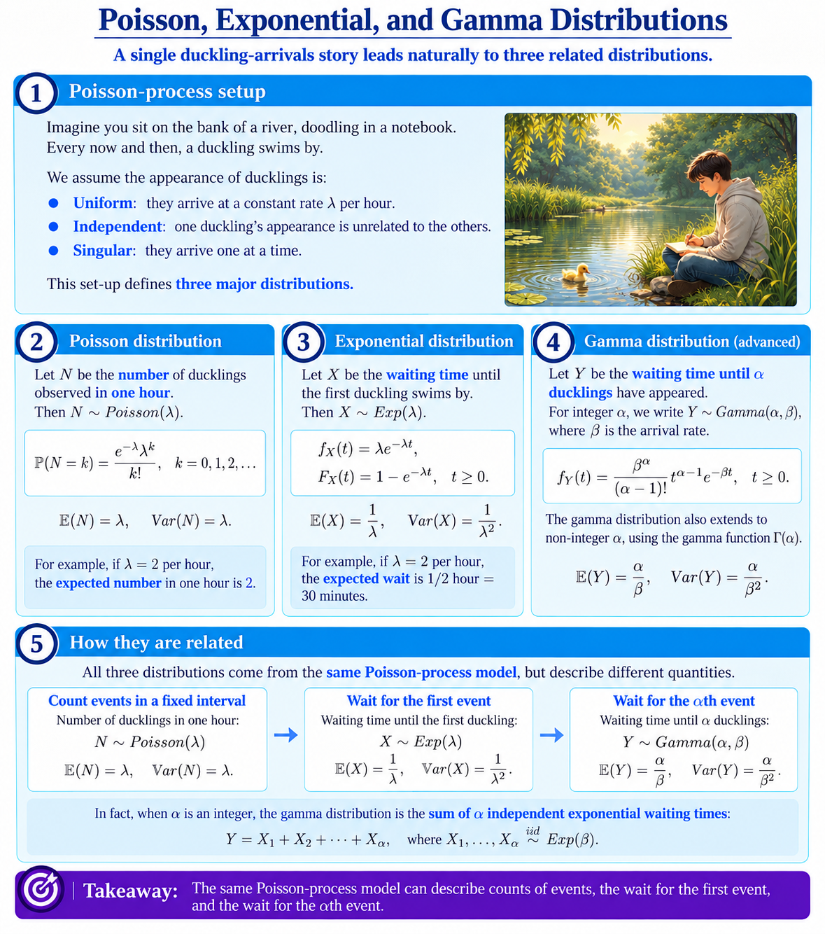
The Poisson, exponential and gamma distributions can all arise from the same kind of event process.
Imagine sitting beside a river reading, and waiting for some ducklings to swim past. Suppose that they arrive at a constant average rate, independently of one another, and only one at a time.
In this situation, we can ask three different questions:
-
How many ducklings appear during a fixed period of time?
-
How long do we wait for the first duckling?
-
How long do we wait for several ducklings to appear?
The answers to these three questions lead us naturally to the Poisson, exponential and gamma distributions.
Poisson Distribution
The Poisson distribution counts the number of events that occur during a fixed interval.
Suppose ducklings arrive at an average rate of $\lambda$ per hour, and let $N$ be the number that appear during one hour. Then
$$N\sim\operatorname{Poisson}(\lambda).$$
The possible values are
$$0,1,2,\dots$$
since we might (sadly) see no ducklings, or one duckling, two ducklings, and so on.
The pmf is:
$$\mathbb{P}(N=k)=\frac{e^{-\lambda}\lambda^k}{k!},$$
for $k=0,1,2,\dots$.
The mean and variance are particularly simple:
$$\mathbb{E}(N)=\lambda,$$
and
$$\operatorname{Var}(N)=\lambda.$$
So if ducklings arrive at an average rate of $2$ per hour, the expected number observed in one hour is also $2$.
The parameter $\lambda$ determines both the location and spread of the distribution. Larger values of $\lambda$ shift the probability towards larger counts.
Explore the Poisson pmf
In the interactive graph below, change $\lambda$ to see how the Poisson distribution changes.
The horizontal axis shows the number of events, $k$, and each bar has height $\mathbb{P}(N=k)$.
You can also choose a particular value of $k$ to calculate the corresponding probability $\mathbb{P}(N=k)$.
Exponential Distribution
Instead of counting how many events occur within a period, suppose we measure how long we have to wait for the first event. For obvious reasons, we call this a “waiting time”!
If events occur at rate $\lambda$, and $X$ is the waiting time until the first event, then
$$X\sim\operatorname{Exp}(\lambda).$$
The exponential distribution is continuous, with pdf
$$f_X(x)=\lambda e^{-\lambda x},\qquad x\geq0.$$
Its cdf is
$$F_X(x)=1-e^{-\lambda x},\qquad x\geq0.$$
The mean is
$$\mathbb{E}(X)=\frac{1}{\lambda},$$
and the variance is
$$\operatorname{Var}(X)=\frac{1}{\lambda^2}.$$
For example, if ducklings arrive at a rate of $\lambda=2$ per hour, then
$$\mathbb{E}(X)=\frac{1}{2}\text{ hour}=30\text{ minutes}.$$
So a higher arrival rate means a shorter expected waiting time.
The exponential distribution is also memoryless. If we have already waited for some time without an event occurring, this does not change the distribution of the additional waiting time.
In symbols,
$$\mathbb{P}(X>s+t\mid X>s)=\mathbb{P}(X>t).$$
Explore the Exponential pdf and Calculate Probabilities
In the interactive graph below, $\lambda$ determines the rate of the exponential distribution.
You can also choose two values, $c$ and $d$, to calculate
$$\mathbb{P}(c\leq X\leq d).$$
The blue shaded region shows this probability as an area under the pdf.
Try changing $\lambda$ and notice how a larger rate concentrates the distribution closer to zero.
Gamma Distribution
The gamma distribution extends the same waiting-time idea from the exponential distribution.
Suppose events occur independently at a constant rate $\beta>0$, and let $\alpha$ be a positive integer. Note that we now use $\beta$ instead of $\lambda$.
Now, let $Y$ be the time we need to wait until the $\alpha$-th event occurs – for instance, until we observe $\alpha$ ducklings. Then we have:
$$Y\sim\operatorname{Gamma}(\alpha,\beta).$$
For example:
-
$\alpha=1$ gives the waiting time until the first event;
-
$\alpha=2$ gives the waiting time until the second event; i.e., the total time needed to observe $2$ ducklings.
-
$\alpha=5$ likewise gives the waiting time until the fifth event.
For a positive integer $\alpha$, the pdf is
$$f_Y(y)=\frac{\beta^\alpha}{(\alpha-1)!}y^{\alpha-1}e^{-\beta y},\qquad y\geq0.$$
The mean is
$$\mathbb{E}(Y)=\frac{\alpha}{\beta},$$
and the variance is
$$\operatorname{Var}(Y)=\frac{\alpha}{\beta^2}.$$
When $\alpha=1$, the pdf becomes
$$f_Y(y)=\beta e^{-\beta y},$$
so the exponential distribution is the special case of the gamma distribution where $\alpha=1$.
A gamma random variable with integer $\alpha$ can also be viewed as the sum of $\alpha$ independent exponential waiting times:
$$Y=X_1+X_2+\cdots+X_\alpha,$$
where $X_1,\dots,X_\alpha$ are independent exponential random variables with rate $\beta$.
That is, to find the total waiting time to spot $\alpha$ ducklings, we add the times we waited for each one, after the previous duckling came along.
Gamma Distributions with Non-Integer $\alpha$
The gamma distribution can also be defined when $\alpha$ is not an integer.
In this more general case, $\alpha$ can be any positive real number:
$$\alpha>0.$$
If $\alpha$ is not an integer, it no longer literally represents the number of events we are waiting for. Instead, $\alpha$ is a shape parameter which controls the shape of the distribution.
To extend the pdf to non-integer values of $\alpha$, we replace the factorial $(\alpha-1)!$ with the gamma function
$$\Gamma(\alpha)=\int_0^\infty t^{\alpha-1}e^{-t}dt.$$
The pdf is then
$$f_Y(y)=\frac{\beta^\alpha}{\Gamma(\alpha)}y^{\alpha-1}e^{-\beta y},\qquad y\geq0.$$
For positive integers, the gamma function satisfies
$$\Gamma(\alpha)=(\alpha-1)!,$$
so this formula agrees exactly with the integer-$\alpha$ version above.
The mean and variance remain
$$\mathbb{E}(Y)=\frac{\alpha}{\beta}$$
and
$$\operatorname{Var}(Y)=\frac{\alpha}{\beta^2}.$$
Here, $\beta$ is the rate parameter. Another common parameterisation instead uses the scale parameter
$$\theta=\frac{1}{\beta}.$$
So it is worth checking whether a source is using a rate or a scale parameter when working with gamma distributions.
Explore the Gamma pdf and Calculate Probabilities
In the interactive graph below, $\alpha$ controls the shape of the gamma distribution and $\beta$ controls its rate.
You can also choose two values, $c$ and $d$, to calculate
$$\mathbb{P}(c\leq Y\leq d).$$
The shaded region shows this probability as an area under the pdf.
Try changing $\alpha$ and $\beta$ to see how the shape and spread of the distribution change.
In particular, when $\alpha=1$, the gamma distribution becomes an exponential distribution.
Background:
Poisson, Exponential and Gamma Summary
| Distribution | What it describes | Parameters | Mean | Variance |
|---|---|---|---|---|
| Poisson | Number of events in a fixed interval | $\lambda$ | $\lambda$ | $\lambda$ |
| Exponential | Waiting time until the first event | $\lambda$ | $1/\lambda$ | $1/\lambda^2$ |
| Gamma | Waiting time until the $\alpha$-th event when $\alpha$ is an integer | $\alpha,\beta$ | $\alpha/\beta$ | $\alpha/\beta^2$ |