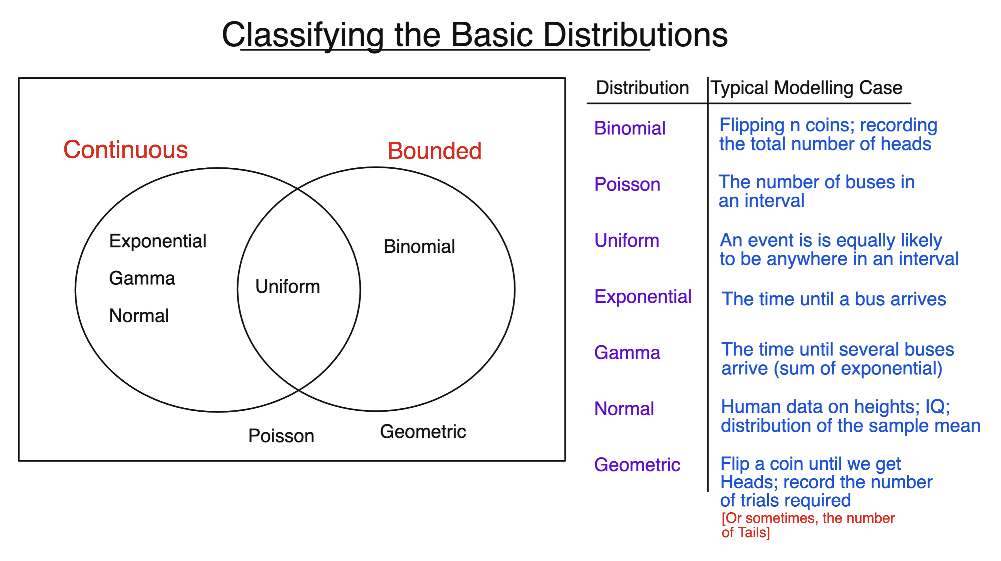
How Can We Identify Which Distribution We Have?
A useful way to recognise a common probability distribution is to remember a typical prototype for when it arises.
For example, a binomial distribution is like flipping a coin a fixed number of times and counting the number of heads.
The situation does not literally have to involve coins. We might instead fire an arrow at a target several times and count the number of hits. What matters is that the underlying structure is the same.
So, when trying to identify a distribution, it is often useful to ask:
-
What kind of quantity are we recording?
-
What familiar prototype does the situation resemble?
We can then narrow things down further by asking whether the distribution is discrete or continuous, and whether it is bounded or unbounded.
Discrete or Continuous?
A discrete distribution describes a random variable with a countable set of possible values.
For the distributions considered here, probabilities of particular values are found using a pmf.
Examples include:
-
the binomial distribution, which counts successes in a fixed number of trials;
-
the Poisson distribution, which counts events in an interval;
-
the geometric distribution, which counts how many trials are needed to obtain the first success.
A continuous distribution instead has a pdf, and probabilities for intervals are found from areas under the pdf.
Examples include:
-
the uniform distribution;
-
the exponential distribution;
-
the gamma distribution;
-
the normal distribution.
Bounded or Unbounded?
A distribution is bounded if all its possible values lie between two fixed finite limits.
For example, if
$$X\sim\operatorname{Bin}(n,p),$$
then
$$X\in{0,1,\dots,n},$$
so the binomial distribution is bounded – below by $0$, and above by $n$.
Similarly, if
$$X\sim\mathcal{U}[a,b],$$
then $X$ must lie between $a$ and $b$.
The other basic distributions considered here are unbounded in at least one direction.
For example, a Poisson random variable can in principle take any non-negative integer value, while a normal random variable can take any real value.
The exponential, gamma and geometric distributions all have a lower limit, but no finite upper limit.
Typical Modelling Cases
The following prototypes are useful to keep in mind:
| Distribution | Type | Bounded? | Typical modelling case |
|---|---|---|---|
| Binomial | Discrete | Yes | Repeat a fixed number of success-or-failure trials and count the successes |
| Poisson | Discrete | No | Count the number of events occurring in a fixed interval |
| Geometric | Discrete | No | Repeat trials until the first success and count how many trials were needed |
| Uniform | Continuous | Yes | Values are spread uniformly across a fixed interval |
| Exponential | Continuous | No | Measure the waiting time until the first event |
| Gamma | Continuous | No | Measure the waiting time until several events have occurred |
| Normal | Continuous | No | Model a symmetric, bell-shaped quantity such as some human characteristics or an approximately normal sample mean |
The prototype is usually the most useful starting point. The discrete/continuous and bounded/unbounded classifications then provide extra clues if you are unsure about this.
Background:
Understanding Econometrics is completely free to use, and always will be.
If you found the site useful and would like to help me keep adding new material, please consider buying me a coffee! Buy me a coffee ☕