The Central Limit Theorem in Action

On the previous page, we saw that the Central Limit Theorem tells us that, for large $n$, the standardised sample mean

$$\frac{\bar X-\mu}{\sigma/\sqrt{n}}$$

has an approximately standard normal distribution.

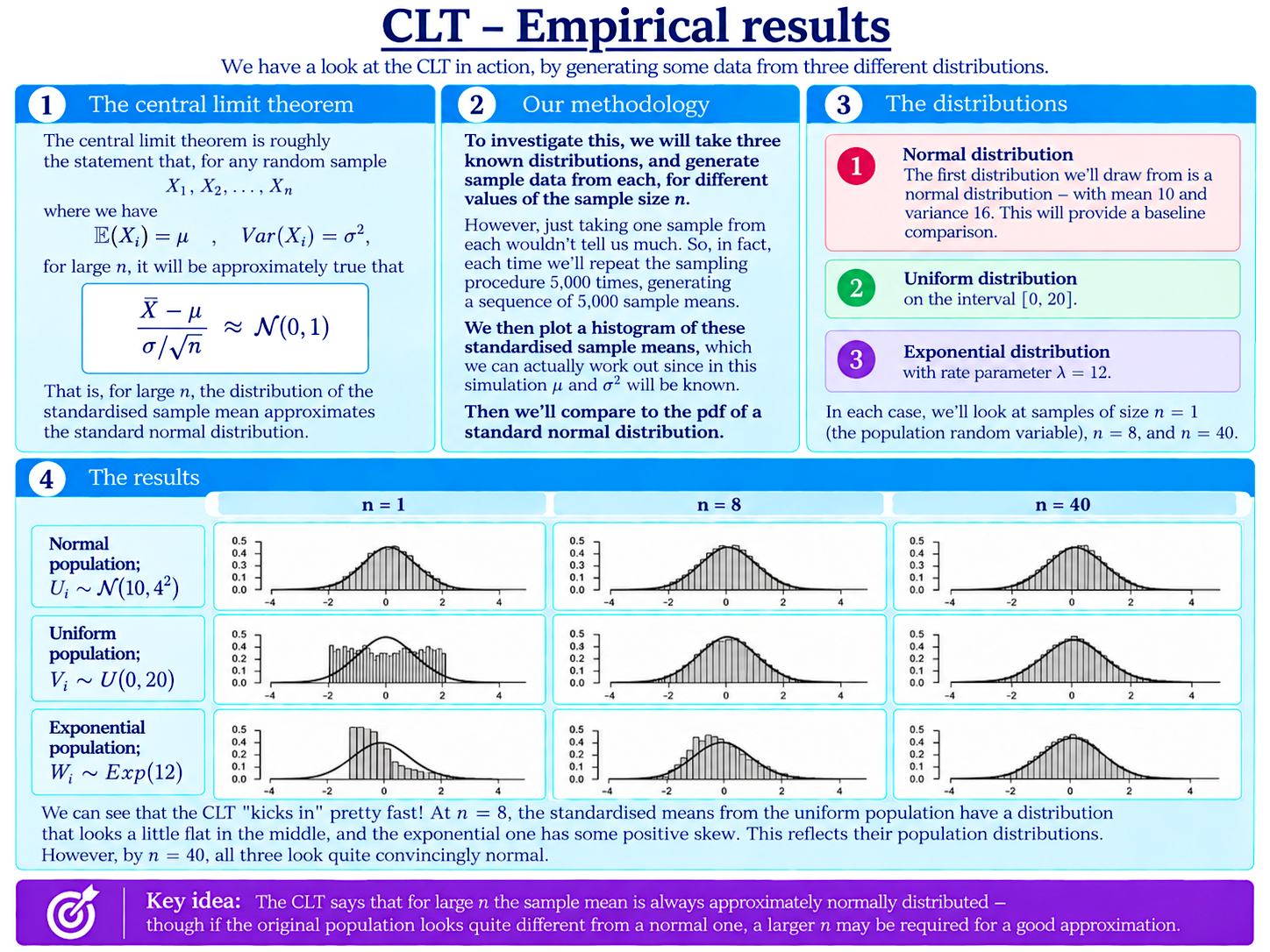
The graphs above let us watch this happen.

We begin with three very different population distributions:

• a normal distribution with mean $10$ and variance $16$;
• a uniform distribution on the interval $[0,20]$;
• an exponential distribution with rate parameter $\lambda=12$.

For each population, we generate random samples of size $n=1$, $n=8$, and $n=40$.

One sample would not tell us much about the distribution of the sample mean. So, for each case, we repeat the sampling procedure $5,000$ times, calculate and standardise the sample mean each time, and plot a histogram showing all $5,000$ resulting values.

The smooth curve shown over each histogram is the pdf of a standard normal distribution.

What Do the Results Show?

The first column, with $n=1$, essentially reproduces the shape of each original population. The normal population is already bell-shaped, the uniform population is flat, and the exponential population is strongly skewed.

By $n=8$, something interesting has already happened to the latter two distributions.

The standardised means from the uniform population remain a little flat in the middle, and the exponential case still retains some positive skew. However, both are beginning to look normal.

By $n=40$, all three distributions of sample means look convincingly normal!

This is the Central Limit Theorem made visible: as the sample size increases, the sample mean progressively loses the distinctive “personality” of the original population and takes on the familiar normal shape.

The graphs also show why there is no universal rule for how large $n$ must be for the normal approximation to be reasonable. A population that is already normal needs no approximation at all, while a population with a more distinctive shape may require a larger sample before the normal approximation becomes convincing.

Notice also that in the first row, the histogram doesn’t become closer to the standard normal as we increase $n$. In this case, the standardised sample mean is already exactly

$$\frac{\bar X-\mu}{\sigma/\sqrt{n}}\sim\mathcal{N}(0,1)$$

for every $n$. Increasing the sample size cannot improve this. The small differences between the histogram and the smooth curve are simply random variation from our simulation.

An Exact Look at the Exponential Case

Finally, let’s explore a little further with the exponential distribution.

Let

$$X_i\sim\operatorname{Exp}(\lambda),$$

and consider again the standardised sample mean for $n$ observations:

$$Z_n=\frac{\bar X-\mu}{\sigma/\sqrt{n}}.$$

The interactive graph below compares the exact pdf of this distribution (in red) with the standard normal distribution (in purple).

For small $n$, the positive skew inherited from the exponential population is very obvious. As $n$ grows, the two curves become increasingly difficult to distinguish.

Even at $n=100$, a little positive skew remains visible. Try changing the value of $n$ manually to something much larger, and see how large the sample needs to become before you can barely tell the two curves apart!

Background

• Uniform Distribution

• Normal Distribution

• Poisson, Exponential, and Gamma Distributions