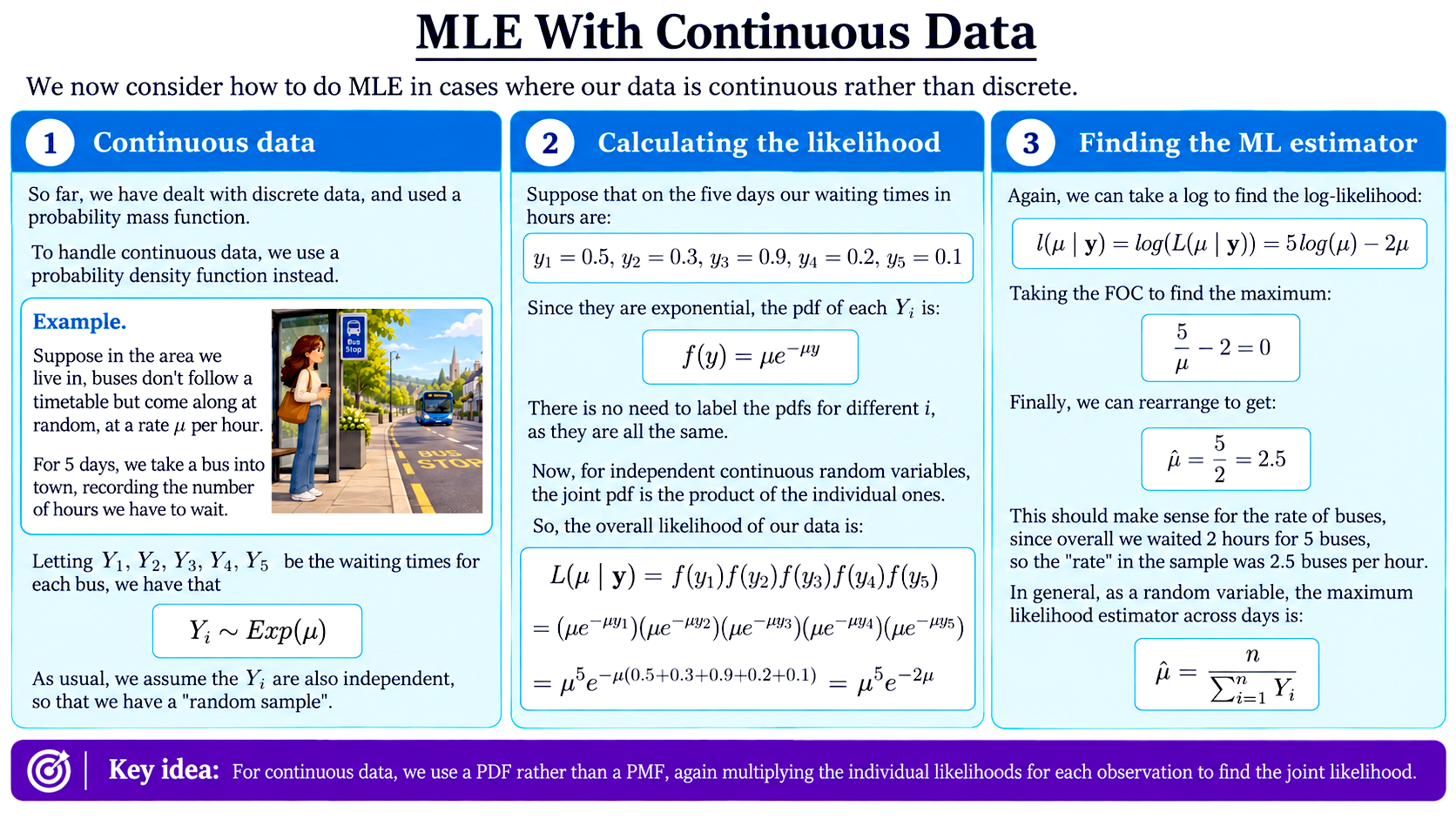
MLE With Continuous Data

So far, our maximum likelihood examples have involved discrete random variables. In these cases, the likelihood was built from probabilities such as

$$\mathbb{P}(X_i=x_i).$$

For a continuous random variable, the probability of observing any one exact value is $0$. So instead, we use the value of the pdf at each observed data point. Of course, for independent random variables, we still multiply the individual “marginal” pdfs to find the joint one.

So, if $Y_1,Y_2,\dots,Y_n$ are continuous and form a random sample, with common pdf $f(y\mid\theta)$, we now define the joint likelihood as

$$L(\theta\mid\mathbf{y})\ = \ f(y_1\mid\theta) \ f(y_2\mid\theta) \ \dots \ f(y_n\mid\theta),$$

where $\theta$ is the unknown parameter.

Apart from this change from probabilities to densities, the idea of maximum likelihood estimation is exactly the same.

Example: Waiting for Buses

Suppose buses arrive randomly at a rate of $\mu$ buses per hour.

The waiting time $Y_i$ for each bus then has an exponential distribution:

$$Y_i\sim\operatorname{Exp}(\mu),$$

with pdf

$$f(y)=\mu e^{-\mu y}.$$

Suppose that over five days we record the waiting times

$$y_1=0.5,\qquad y_2=0.3,\qquad y_3=0.9,\qquad y_4=0.2,\qquad y_5=0.1.$$

Because the observations are independent, the joint likelihood is the product of the five densities:

$$L(\mu\mid\mathbf{y})=(\mu e^{-\mu y_1})(\mu e^{-\mu y_2})(\mu e^{-\mu y_3})(\mu e^{-\mu y_4})(\mu e^{-\mu y_5}).$$

The waiting times add up to $2$ hours, giving

$$L(\mu\mid\mathbf{y})=\mu^5e^{-2\mu}.$$

Finding the Maximum Likelihood Estimate

As before, it is easier to maximise the log-likelihood:

$$l(\mu\mid\mathbf{y})=5\log(\mu)-2\mu.$$

Differentiating and setting the result equal to $0$ gives

$$\frac{5}{\mu}-2=0.$$

Hence,

$$\hat\mu=\frac{5}{2}=2.5.$$

This result has a natural interpretation. Across our five journeys, we waited for a total of $2$ hours, so the observed rate was

$$\frac{5}{2}=2.5$$

buses per hour.

For a general random sample of exponential waiting times, the maximum likelihood estimator is

$$\hat\mu=\frac{n}{\sum_{i=1}^nY_i}=\frac{1}{\bar Y}.$$

So, although we have moved from discrete to continuous data, the basic method has not changed: construct the likelihood from the data, then choose the parameter value that maximises it.

Background

• Poisson, Exponential, and Gamma Distributions