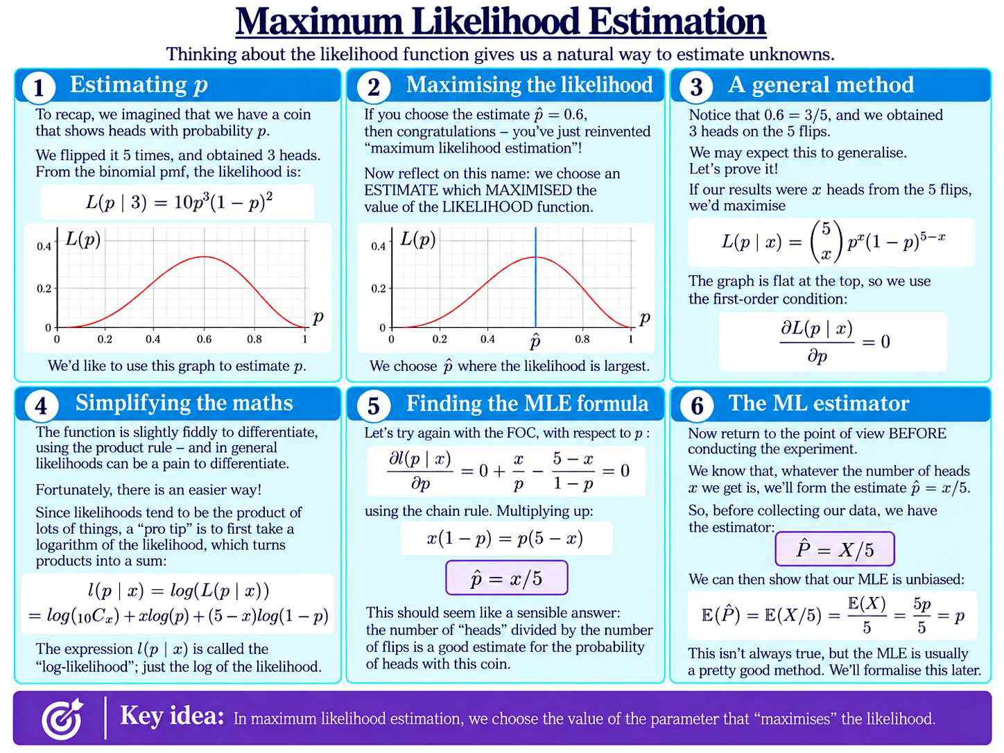
What Is Maximum Likelihood Estimation?

On the previous page, we imagined flipping a coin five times and observing three heads.

If $p$ is the unknown probability of heads, the likelihood of our result is

$$L(p\mid 3)=10p^3(1-p)^2.$$

The graph in Box 1 of this slide plots this likelihood for different possible values of $p$.

Now, suppose you are invited to guess $p$ based on the graph.

If you chose

$$\hat p=0.6$$

as your estimate, then congratulations – you have just re-invented maximum likelihood estimation!

The idea is exactly what the name suggests: choose the value of the unknown parameter that maximises the likelihood of the data we actually observed.

Finding Maximum Likelihood Estimates

Suppose more generally that we obtain $x$ heads from our five coin flips.

The likelihood is then

$$L(p\mid x)=\binom{5}{x}p^x(1-p)^{5-x}.$$

To find the maximum likelihood estimate, we look for the value of $p$ at which this function is largest.

In principle, we could differentiate the likelihood directly and use the usual first-order condition

$$\frac{\partial L(p\mid x)}{\partial p}=0.$$

But likelihood functions can quickly become awkward to differentiate.

Fortunately, there is a useful trick.

The Log-Likelihood

Instead of maximising the likelihood itself, we can maximise its logarithm.

We define the log-likelihood

$$l(p\mid x)=\log(L(p\mid x)).$$

For our binomial example,

$$l(p\mid x)=\log\binom{5}{x}+x\log(p)+(5-x)\log(1-p).$$

Taking logs is helpful because products and powers turn into sums and multiples, making the expression much easier to differentiate.

It also does not change where the maximum occurs, since the logarithm is an increasing function.

Differentiating with respect to $p$ gives

$$\frac{\partial l(p\mid x)}{\partial p}=\frac{x}{p}-\frac{5-x}{1-p}.$$

Setting this equal to $0$,

$$\frac{x}{p}-\frac{5-x}{1-p}=0,$$

and rearranging gives

$$\hat p=\frac{x}{5}.$$

So the maximum likelihood estimate is simply the proportion of our five flips that came up heads.

For the result $x=3$,

$$\hat p=\frac{3}{5}=0.6,$$

exactly as the graph suggested.

From the Estimate to the Estimator

So far, $x$ has represented the number of heads we actually observed.

Before performing the experiment, however, the number of heads is the random variable $X$. The corresponding maximum likelihood estimator is therefore

$$\hat P=\frac{X}{5}.$$

Notice that we have now switched back to a probability perspective. By thinking of our estimator as a random variable before collecting the data, we can use probability theory to investigate how good our statistical method is.

In this example, the estimator is unbiased:

$$\mathbb{E}(\hat P)=\mathbb{E}\left(\frac{X}{5}\right)=\frac{\mathbb{E}(X)}{5}=\frac{5p}{5}=p.$$

This is a nice property of our estimator here. Maximum likelihood estimators are not automatically unbiased in general, though later we will discuss an interesting result in this area.

Background

• Binomial Distribution