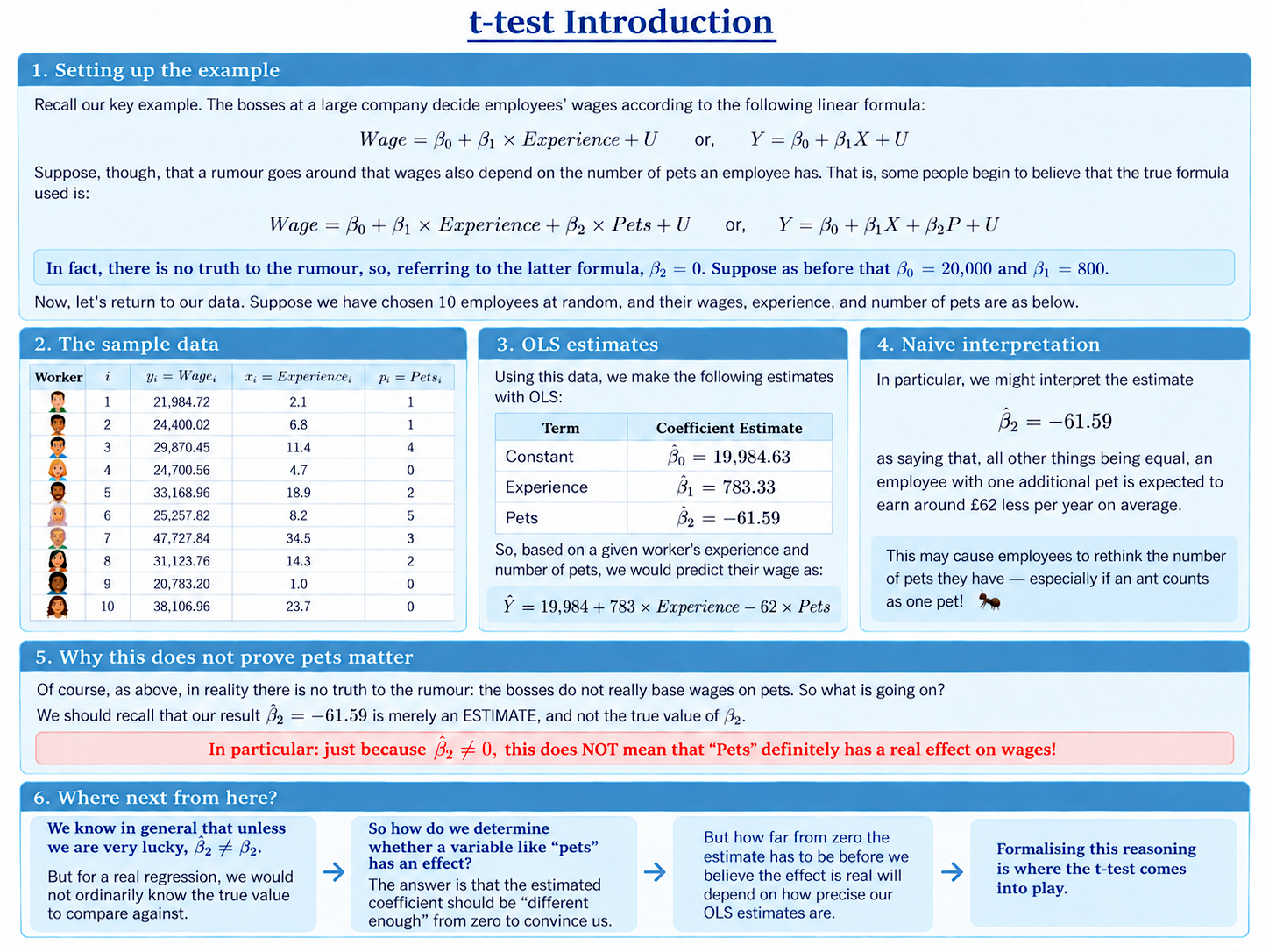
Why Do We Need a $t$-test?

Suppose we have a simple linear model:

$$Y=\beta_0+\beta_1X+U$$

We would like to know whether $X$ has an effect on $Y$. This will be true whenever $\beta_1$ is not equal to zero.

Now, suppose we estimate the regression model and obtain a coefficient estimate

$$\hat\beta_1$$

Perhaps the estimate is positive. Perhaps it is negative. Either way, a tempting conclusion is that, since $\hat\beta_1\neq0$, $X$ must genuinely have an effect on $Y$.

Unfortunately, things are not quite that easy!

Estimates Are Not the True Coefficients

The quantity $\hat\beta_1$ is only an estimate of the unknown population coefficient $\beta_1$.

Different random samples generally give us different estimates.

So even if the true coefficient were

$$\beta_1=0$$

we would not usually expect our particular sample to produce exactly

$$\hat\beta_1=0$$

We might instead obtain a small positive estimate, a small negative estimate, or occasionally something rather further from zero.

In particular, the fact that $\hat\beta_1\neq0$ does not by itself show that $\beta_1\neq0$!

However, if $\hat\beta_1$ is very far from zero, we might start to doubt whether the real $\beta_1$ can still be zero after all. We are proud of our little OLS method, after all, and hope it gives reasonably accurate estimates!

This thought is the intuition behind the $t$-test.

How Far From Zero Is Far Enough?

This leads to the key question:

How far from zero does our estimate $\hat\beta_1$ need to be before we have convincing evidence that the true coefficient $\beta_1$ is not zero?

Unfortunately, the question is a little tricky.

Suppose our model is

$$Wage=\beta_0+\beta_1Age+U$$

Now suppose we transform the model and our dataset so that, instead of measuring $Wage$ in dollars, we now measure it in cents.

Since everything on the left-hand side of our equation gets 100 times bigger, the same thing must happen on the right-hand side. For instance, $\beta_0$ will be replaced with $100\beta_0$. And since we are not changing how we measure age, $\beta_1$ will need to be 100 times bigger too.

Likewise, in our data, the best-fitting model will have an estimate $\hat\beta_1$ that is 100 times bigger. Yet nothing substantive about the relationship between age and wages has changed at all!

As we see here, the actual size of the number we get for $\hat\beta_1$ can essentially be manipulated at will by changing units. Therefore, there cannot be a “one-size-fits-all” rule for how large the estimate needs to be.

The trick is to think relative to how precise our estimator is.

That is, an estimate that looks quite far from zero may not be very surprising, even if there is no true effect, if the estimator itself is quite imprecise, and varies all over the place.

On the other hand, even a fairly modest departure from zero may be persuasive if the estimator is very precise!

Ideally, we would measure the precision of an estimator using its variance or standard deviation. Since we do not know either of these, in the $t$-test we will instead use its standard error – our estimate of its standard deviation.

Background

• Unbiasedness
• Gauss-Markov – Part I