Testing a Coefficient Against Another Value

So far, we have practised using a $t$-test to determine whether a regression coefficient is equal to zero.

But there is nothing special about the number zero. In fact, a $t$-test can also be used to test whether a coefficient is equal to any particular value.

Let’s see how this works.

The Model and the Question

Suppose an economist is interested in the relationship between household consumption and income across countries.

They specify the population model

$$C=\beta_0+\beta_1Y+U$$

where $C$ is consumption and $Y$ is income.

Using data from 30 countries, they estimate

$$\widehat{C}=-2982.276+0.823Y$$

with

$$SE(\hat\beta_1)=0.0376$$

We would like to test whether $\beta_1$, the “marginal propensity to consume”, is equal to one.

So, our hypotheses are

$$H_0:\beta_1=1$$

and

$$H_1:\beta_1\neq1$$

Notice the important difference from our previous example: the null hypothesis now claims that the coefficient is one, rather than zero.

Of course, our estimate $\hat\beta_1$ is $0.823$ rather than $1$; but since this is just an estimate, we know it is not conclusive by itself.

The Test Statistic

In general, when testing

$$H_0:\beta_j=c$$

we use the test statistic

$$T=\frac{\hat\beta_j-c}{SE(\hat\beta_j)}$$

So here,

$$T=\frac{\hat\beta_1-1}{SE(\hat\beta_1)}$$

We use this statistic because, if the null is true and indeed $\beta_j=c$, then $T$ becomes exactly our standardised estimator:

$$T=\frac{\hat\beta_j-\beta_j}{SE(\hat\beta_j)}\sim t_{n-k-1}$$

In our example, the sample contains $n=30$ countries and the model has $k=1$ independent variable, so under the null

$$T\sim t_{28}$$

Of course, all of this is still conditional on $\mathbf{X}=\mathbf{x}$, but we suppress this notation now that we’re hopefully comfortable with what is going on.

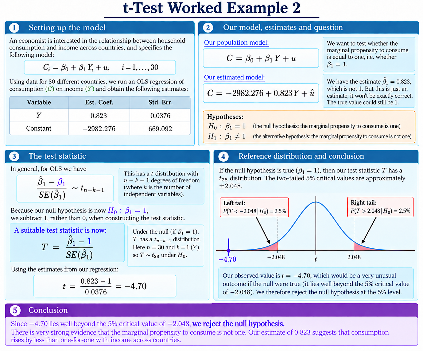
Using our estimates, we find the observed value $t$:

$$t=\frac{0.823-1}{0.0376}=-4.70$$

Our estimate is therefore about 4.7 standard errors below the value of one claimed by the null hypothesis. Hmmm – suspicious!

Conducting the Test

We know that, if the null hypothesis is true, then

$$T\sim t_{28}$$

For a two-tailed test at the 5% significance level, the critical values are approximately

$$-2.048\qquad\text{and}\qquad2.048$$

That is, under the null, there is only a 5% chance that $T$ falls either below $-2.048$ or above $2.048$.

However, our observed value of $T$ in the sample is

$$t=-4.70$$

This lies well beyond the lower critical value, as shown in the graph above.

Conclusion

We therefore reject the null hypothesis

$$H_0:\beta_1=1$$

at the 5% significance level.

The data provide strong evidence that the marginal propensity to consume is not equal to one.

Moreover, since our estimate is

$$\hat\beta_1=0.823$$

the estimated relationship suggests that consumption rises by less than one-for-one with income across the countries in our sample.

The important extension from the previous example is straightforward: when the null hypothesis claims some value other than zero, we simply subtract that value (rather than zero) when constructing the test statistic $T$.