Testing Whether a Coefficient Is Zero

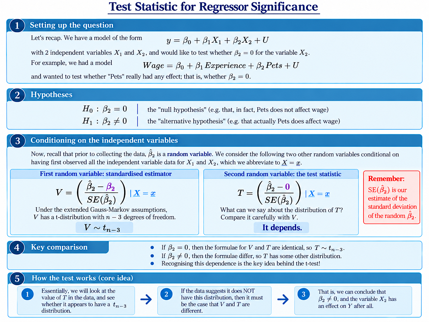
Suppose we have a regression model with two independent variables:

$$Y=\beta_0+\beta_1X_1+\beta_2X_2+U$$

We would like to test whether $X_2$ really has an effect on $Y$.

In terms of the population coefficient, our question is whether

$$\beta_2=0$$

or whether

$$\beta_2\neq0$$

We formalise these two possibilities using hypotheses.

The Null and Alternative Hypotheses

Our null hypothesis is

$$H_0:\beta_2=0$$

while our alternative hypothesis is

$$H_1:\beta_2\neq0$$

The null hypothesis is therefore the claim that $X_2$ has no effect on $Y$ in our population model.

A Standardised Estimator

Recall that $\hat\beta_2$ is a random variable before we collect our data.

Conditional on the observed independent-variable data $\mathbf{X}=\mathbf{x}$, consider the standardised estimator

$$V= \left( \frac{\hat\beta_2-\beta_2}{SE(\hat\beta_2)} \right) _{\mid \mathbf{X}=\mathbf{x}} $$

$V$ is a useful thing to think about because, under our full set of regression assumptions, including normality, $V$ is a “pivot” – a random variable whose distribution is fully known.

More specifically, under these standard assumptions, $V$ always has a $t$-distribution with $n-k-1$ degrees of freedom (for a sample size $n$ and model with $k$ independent variables).

In the example on the slide, then, since the model has two independent variables and an intercept,

$$V\sim t_{n-3}$$

Let’s continue with this example for the rest of the slide; the extension to the general case should be clear.

The Test Statistic

The random variable that is the star of the show with the $t$-test is given by the following formula. We call it the test statistic:

$$T= \left( \frac{\hat\beta_2-\color{red}{0}}{SE(\hat\beta_2)} \right) _{\mid \mathbf{X}=\mathbf{x}} $$

Now, compare this very carefully with $V$:

$$V= \left( \frac{\hat\beta_2-\color{red}{\beta_2}}{SE(\hat\beta_2)} \right) _{\mid \mathbf{X}=\mathbf{x}} $$

Are they the same, or different? Or does it depend? Be as precise as you can!

The Key Comparison

In comparing $V$ and $T$ we should have noticed that they were almost the same, except that in the formula for $T$, the $\beta_2$ has been replaced with a $0$.

So, is $T$ different from $V$? The answer is: it depends.

Recall that we don’t know the value of $\beta_2$. It might be $0$; or on the other hand, it might not be. In fact, whether $\beta_2=0$ or not is exactly the thing we are supposed to be testing. Hmmm – interesting!

More formally, we might say that, if the null hypothesis is true, then $\beta_2=0$ – and in that case, the two formulae become identical:

$$T=V$$

Now, we know for sure that $V$ has a $t$-distribution. So, if indeed the null hypothesis is true, and $V$ and $T$ are therefore exactly the same, it will also be true that

$$T\sim t_{n-3}$$

under the null hypothesis.

Let’s repeat that one more time:

$$H_0 \text{ is true } \ \ \Rightarrow \ \ \beta_2=0 \ \ \Rightarrow \ \ T=V \ \ \Rightarrow \ \ T\sim t_{n-3}$$

On the other hand, if the null is false, and $\beta_2\neq0$, then $T$ and $V$ will be different random variables, and $T$ will no longer have this same $t$-distribution, but some other distribution.

This is the central idea behind the test.

How the Test Works

Once we have collected our data, we calculate the observed value of $T$, usually written as a lower-case $t$.

We then ask:

Does this $t$ look like a value that might plausibly have arisen from a $t_{n-3}$ distribution?

Of course, this is exactly the same question as the following:

Does this $t$ look like a value that might plausibly have arisen from the distribution that $T$ would have if $H_0$ were true?

If our observed $t$ is something that would be very unusual under the $t_{n-3}$ distribution, this suggests that perhaps the whole story is bluff and $H_0$ is false after all.

On the next page, we put this method to work in a full example.