The $t$-test: Step by Step
We have now spent some time understanding why the regression $t$-test works.
Fortunately, actually carrying one out is much quicker!
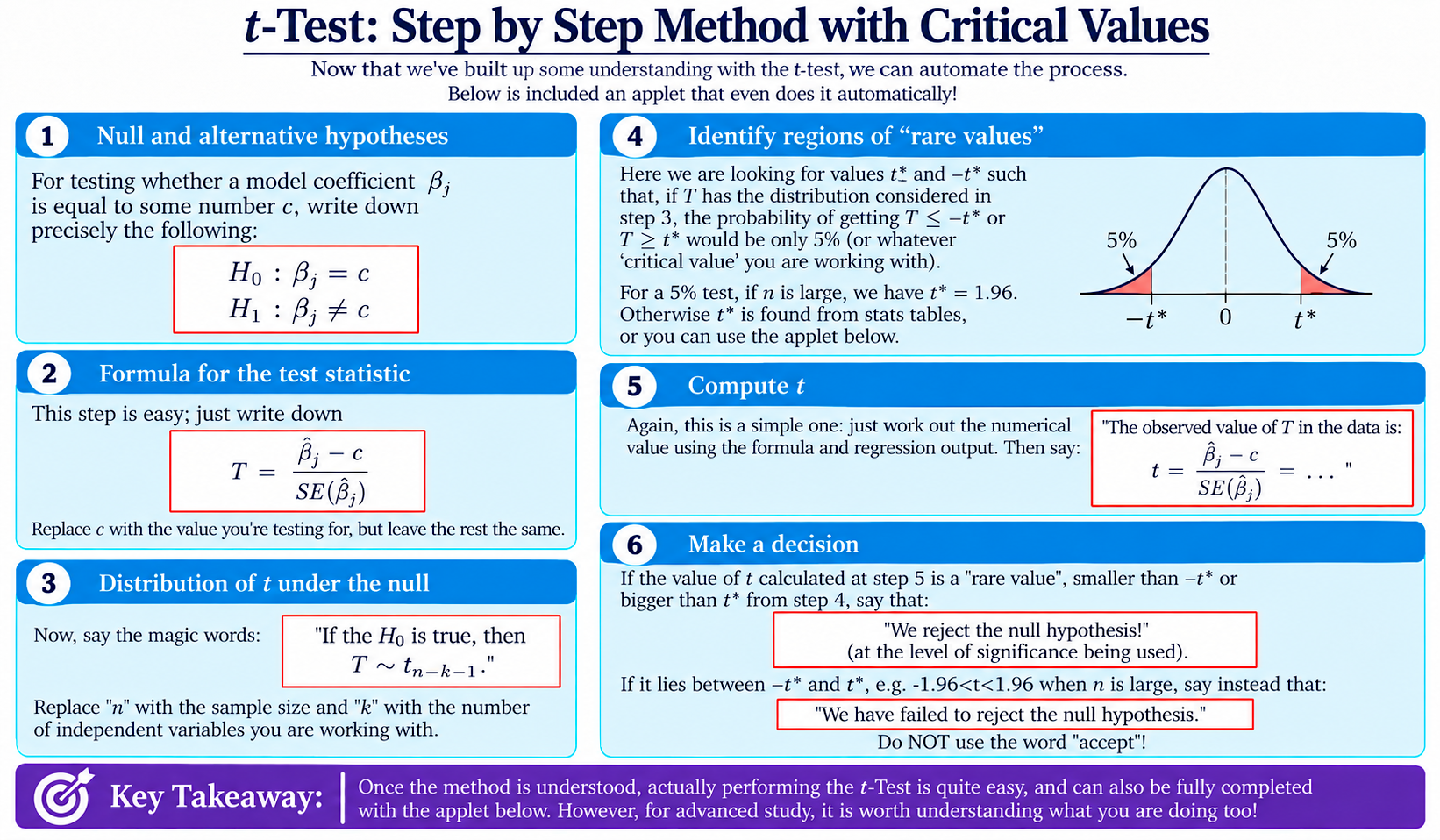
Below is a step-by-step method for a two-tailed $t$-test using critical values, where we want to test whether a regression coefficient $\beta_j$ is equal to some particular value $c$.
In particular, the boxes tell you precisely what to say, after substituting the information from the question you are working on. Then, at the bottom, there is an applet that will conduct the test for you when given this information.
Step 1: State the Hypotheses
First, write down precisely what we are testing.
The null hypothesis claims that the true coefficient is equal to $c$:
$$H_0:\beta_j=c$$
The alternative says that it is different from $c$:
$$H_1:\beta_j\neq c$$
For the familiar test of whether a variable has any effect, $c=0$. But $c$ can be any value.
$H_0:\beta_j=c$
$H_1:\beta_j\neq c$
Replace $j$ with the label of the coefficient you are testing, and $c$ with the value you are testing it against.
Step 2: Write Down the Test Statistic
The test statistic is
$$T=\frac{\hat\beta_j-c}{SE(\hat\beta_j)}$$
$T=\dfrac{\hat\beta_j-c}{SE(\hat\beta_j)}$
Replace $c$ with the value claimed under your null hypothesis, and $j$ with the label of the coefficient you are testing. Everything else stays the same, as written.
Step 3: State the Distribution Under the Null
Now come the magic words:
If $H_0$ is true, then
$$T\sim t_{n-k-1}$$
where $n$ is the sample size and $k$ is the number of independent variables in the regression.
This is the reference distribution we use to judge whether our observed result would be unusual under the null hypothesis.
If $H_0$ is true, then $T\sim t_{n-k-1}$.
Here, substitute the actual values of $n$ and $k$ you are using.
Step 4: Find the Critical Values
Next, identify the values of $t$ that would count as sufficiently rare under the null hypothesis.
For a two-tailed test at significance level $\alpha$, we choose critical values $-t^* $ and $t^* $ so that the total probability in the two tails is $\alpha$.
For a 5% test with a large number of degrees of freedom,
$$t^*\approx1.96$$
For other cases, the appropriate critical value can be obtained from a $t$-table, statistical software, or the applet below.
At significance level $\alpha$, the critical values are $-t^* $ and $t^* $.
Here, replace $\alpha$ with the significance level you are using, and $t^* $ with the correct critical value.
For example:
“At the 5% significance level, the critical values are $-2.048$ and $2.048$.”
Step 5: Calculate the Observed $t$
Now use the coefficient estimate and standard error from the regression output:
$$t=\frac{\hat\beta_j-c}{SE(\hat\beta_j)}$$
Remember that $T$ is the random variable, while lower-case $t$ is the particular value we actually observe in our data.
The observed value of $T$ in the data is
$t=\dfrac{\hat\beta_j-c}{SE(\hat\beta_j)}=\ldots$
Substitute the estimate, the value claimed under the null hypothesis and the standard error from the question, and calculate the numerical value of $t$.
Step 6: Make a Decision
Finally, compare the observed $t$ with the critical values.
If
$$t<-t^*$$
or
$$t>t^*$$
then the observed result lies in one of our rare-event regions. We reject the null hypothesis at the chosen significance level.
"We reject the null hypothesis at significance level $\alpha$."
If, for example, $\alpha=0.05$, write:
“We reject the null hypothesis at the 5% significance level.”
If instead
$$-t^* \leq t \leq t^*$$
then our result is not sufficiently unusual under the null, so we fail to reject it.
"We fail to reject the null hypothesis at significance level $\alpha$."
Again, if $\alpha=0.05$, write:
“We fail to reject the null hypothesis at the 5% significance level.”
Notice the wording. We do not normally say that we “accept” the null hypothesis. Failing to find sufficiently strong evidence against a claim is not the same thing as proving that the claim is true.
Now You Try
The applet below carries out exactly the same method.
You can change the following sliders:
- $\beta_{null}$ – the value of the coefficient claimed under the null hypothesis
- $\beta_{observed}$ – the coefficient estimate observed in the data
- $s_{ErrorBeta}$ – the standard error of the coefficient estimate
- $n$ – the sample size
- $k$ – the number of independent variables
- $\alpha$ – the significance level
The applet then updates the reference distribution, critical values, observed $t$ and conclusion automatically.
Before looking at its conclusion, try to predict whether the null hypothesis will be rejected.