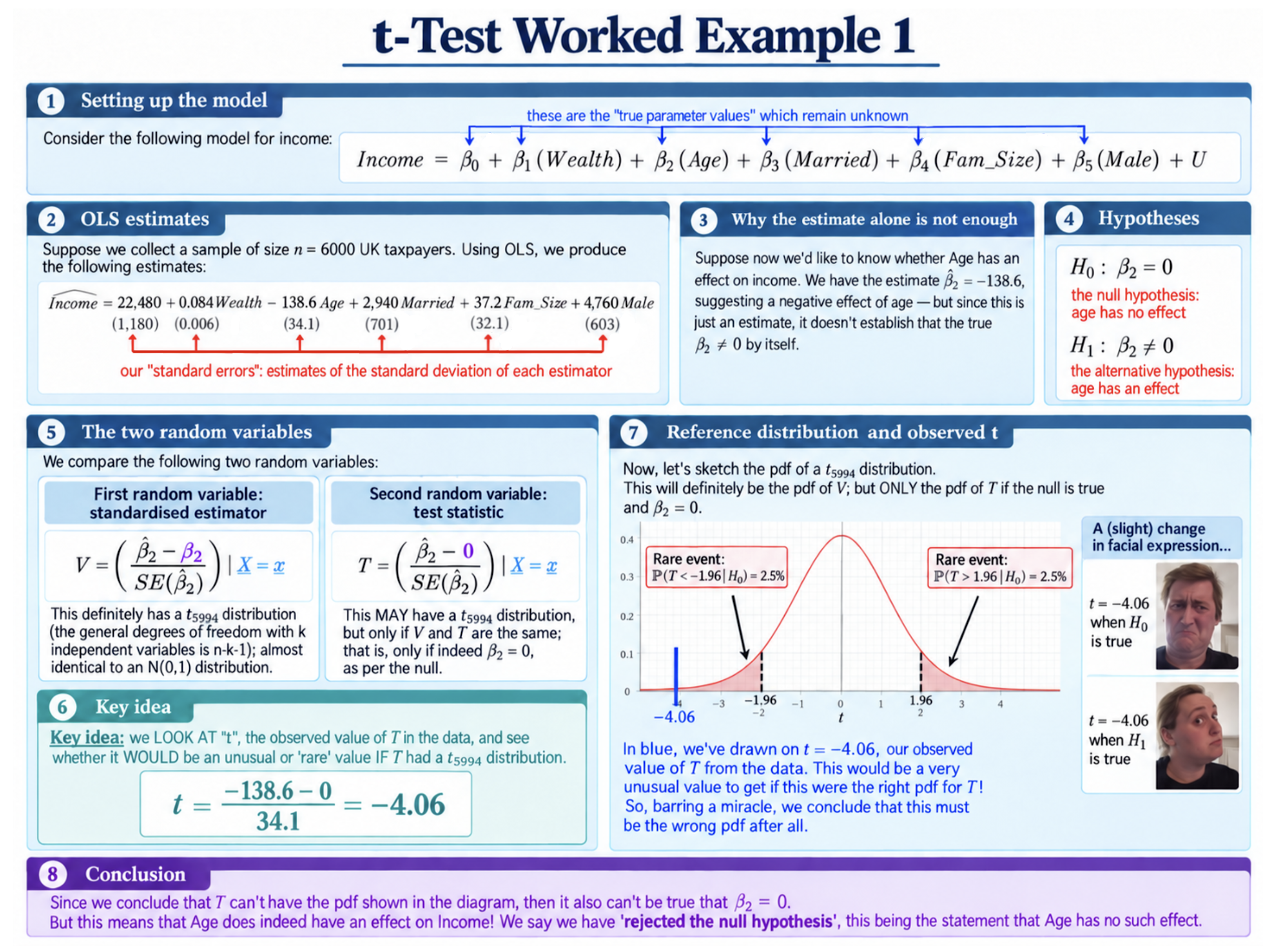
A Worked $t$-test

Let’s now put our $t$-test into practice.

Suppose we are interested in the following population model for income:

$$Income=\beta_0+\beta_1Wealth+\beta_2Age+\beta_3Married+\beta_4Fam_Size+\beta_5Male+U$$

In particular, we would like to know whether $Age$ has an effect on $Income$; that is, whether $\beta_2\neq0$.

We collect a sample of

$$n=6000$$

UK taxpayers and estimate the model using OLS.

Our estimated model is

$$\widehat{Income}=22,480+0.084Wealth-138.6Age+2,940Married+37.2Fam_Size+4,760Male$$

Let’s focus on the coefficient on $Age$:

$$\hat\beta_2=-138.6$$

The negative estimate suggests that, holding the other variables fixed, income decreases with age.

But, as we have emphasised, $\hat\beta_2$ is only an estimate. The fact that it is negative does not by itself establish that the true coefficient $\beta_2$ is different from zero in reality.

Suppose further that we calculate its standard error:

$$SE(\hat\beta_2)=34.1$$

Step 1: State the Hypotheses

Since we are testing whether $Age$ has an effect on $Income$, our null hypothesis is

$$H_0:\beta_2=0$$

and our alternative hypothesis is

$$H_1:\beta_2\neq0$$

So the null says that $Age$ has no effect within our population model, while the alternative says that its coefficient is non-zero.

Step 2: Compare $V$ and $T$

Recall our standardised estimator from the previous page:

$$V=\left(\frac{\hat\beta_2-\color{red}{\beta_2}}{SE(\hat\beta_2)}\right)_{\mid\mathbf{X}=\mathbf{x}}$$

Under our standard regression assumptions, including normality, we know for sure that

$$V\sim t_{n-k-1}$$

Our model contains $k=5$ independent variables, so here

$$V\sim t_{5994}$$

Now consider our test statistic:

$$T=\left(\frac{\hat\beta_2-\color{red}{0}}{SE(\hat\beta_2)}\right)_{\mid\mathbf{X}=\mathbf{x}}$$

If the null hypothesis is true, then

$$\beta_2=0$$

and therefore $V$ and $T$ are exactly the same random variable.

So, under $H_0$,

$$T\sim t_{5994}$$

This $t_{5994}$ distribution may be called our reference distribution for the test.

To emphasise one more time: whether or not $H_0$ is true is precisely the question of whether $T$ has this reference $t_{5994}$ distribution.

Step 3: Calculate the Observed $t$

Once we have collected our particular sample, $T$ takes an observed value $t$.

Using our estimate and standard error,

$$t=\frac{-138.6-0}{34.1}=-4.06$$

So, our observed estimate lies just over four estimated standard deviations below the value of zero claimed by the null hypothesis.

On the slide, this is shown graphically.

Step 4: Is This Plausible Under the Null?

If $H_0$ were true, our observed $t$ would have come from a $t_{5994}$ distribution – which is extremely close to a standard normal distribution.

For a distribution like this, there is only about a 5% chance of getting a value bigger than $1.96$ or less than $-1.96$.

That is, such an occurrence would be a “rare event” at the 5% significance level, our chosen threshold for what counts as sufficiently unusual.

Yet our observed value is far more extreme:

$$t=-4.06$$

If indeed the null were true, and $T\sim t_{5994}$, we would have witnessed an extraordinarily unusual event.

We could put this down to astonishing luck. But the more reasonable explanation is that the story we started with – that $\beta_2=0$ – is false.

Conclusion

Formally, at this point you should say politely that you reject the null hypothesis, $H_0:\beta_2=0$, at the 5% significance level.

What does this actually mean?

It means that the value we observed would be sufficiently unusual if $\beta_2=0$ that the data have convinced us to reject that possibility. We therefore have evidence that $Age$ has an effect on $Income$ within this model.

Of course, our estimate

$$\hat\beta_2=-138.6$$

has suggested all along that this effect is negative, holding the other variables fixed.

But the crucial point is that we did not reject the null merely because $\hat\beta_2$ was different from zero. We rejected it because our observed $t=-4.06$ would be very unusual if $T$ really had the $t_{5994}$ distribution implied by the null hypothesis.

Coming full circle to our initial thoughts at the start of this section, we arrived at $t=-4.06$ by evaluating the coefficient estimate relative to how precise we think our estimator is: that is, by dividing the estimate by its standard error, our estimate of the estimator’s standard deviation.

Background

• Regression $t$-test Introduction
• Test Statistic For Regressor Significance