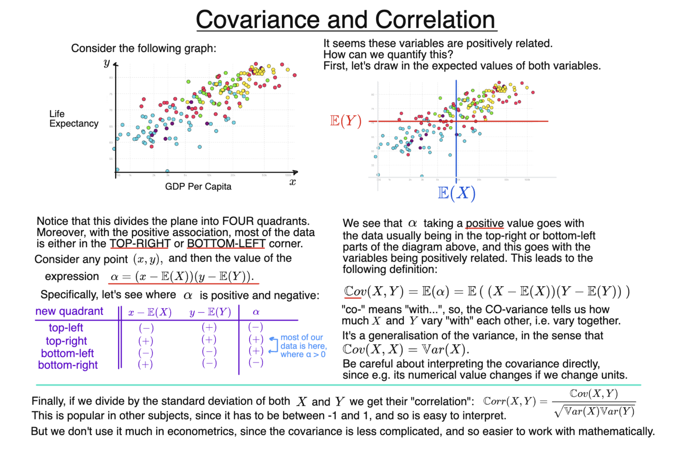
What is Covariance?

The covariance of two random variables measures the extent to which they tend to vary together.

Suppose $X$ and $Y$ are positively related. When $X$ is above its own mean, $Y$ will also tend to be above its mean; and when $X$ is below its mean, $Y$ will tend to be below its mean.

Consider the expression

$$\left(X-\mathbb{E}(X)\right)\left(Y-\mathbb{E}(Y)\right).$$

If both variables are above their means, both brackets are positive, so their product is positive. If both are below their means, both brackets are negative, so the product is again positive.

By contrast, if one variable is above its mean while the other is below, the product is negative.

This leads us to the definition of covariance:

$$\operatorname{Cov}(X,Y)=\mathbb{E}\left(\left(X-\mathbb{E}(X)\right)\left(Y-\mathbb{E}(Y)\right)\right).$$

A positive covariance means that values of $X$ and $Y$ tend to lie on the same side of their respective means. A negative covariance means that they tend to lie on opposite sides.

A covariance of zero means that these positive and negative contributions cancel out on average. This does not necessarily mean that the random variables are unrelated: covariance measures one particular kind of association, and other, nonlinear relationships can still be present when the covariance is zero.

If $X$ and $Y$ are indeed independent, then

$$\operatorname{Cov}(X,Y)=0.$$

However, the converse is not generally true.

An equivalent formula, which is often easier to calculate with, is

$$\operatorname{Cov}(X,Y)=\mathbb{E}(XY)-\mathbb{E}(X)\mathbb{E}(Y).$$

Covariance and Variance

Covariance is closely related to variance. If we take the covariance of a random variable with itself, we get

$$\operatorname{Cov}(X,X)=\operatorname{Var}(X).$$

So, variance can be viewed as a special case of covariance. “Co-” means “with”, so covariance measures the extent to which the two variables “vary together”.

Difficulties in Interpreting Covariance Directly

The numerical size of a covariance depends on the units in which the variables are measured.

For example, suppose $X$ is GDP per capita and $Y$ is life expectancy. If GDP is measured in dollars rather than thousands of dollars, the numerical covariance will be 1000 times as large, even though the underlying relationship has not changed.

This makes the sign of covariance very useful, but its numerical magnitude harder to interpret by itself.

What is Correlation?

The correlation between $X$ and $Y$ rescales their covariance using their standard deviations:

$$\operatorname{Corr}(X,Y)=\frac{\operatorname{Cov}(X,Y)}{\sqrt{\operatorname{Var}(X)\operatorname{Var}(Y)}}.$$

Provided both variables have positive variance, the correlation always lies between $-1$ and $1$.

Unlike covariance, correlation does not change simply because we change the units in which the variables are measured. This makes its numerical value much easier to interpret and compare with other cases.

A positive correlation indicates a positive linear association, while a negative correlation indicates a negative linear association. Values closer to $1$ or $-1$ indicate a stronger linear association, while values closer to $0$ indicate a weaker one.

As with covariance, however, a correlation of zero does not rule out every possible relationship between $X$ and $Y$.

Although correlation is used frequently in other subjects, covariance is particularly useful in econometrics because it behaves very neatly algebraically, and many important properties of interest can be expressed naturally in terms of covariances.

Background:

• Variance and Standard Deviation

Extensions

• Properties of Variance and Covariance