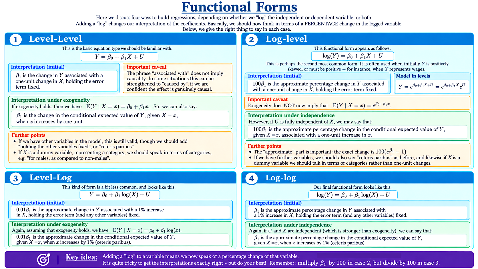
Four Functional Forms
So far, many of our regression models have taken the form
$$Y=\beta_0+\beta_1X+U$$
Here, both $Y$ and $X$ appear in their original units.
However, you may have noticed that some other ways of combining $Y$ and $X$ into a model are also common.
In particular, it is very common to enrich the model by taking the logarithm of $Y$, $X$, or both.
This is not done only to make life more complicated, or to confuse students!
For some variables, percentage changes are more natural and informative than changes in absolute units. For example, an extra £1,000 of income means something rather different to someone earning £10,000 than to someone earning £100,000, whereas a 10% increase has a clearer proportional interpretation.
Taking logs also compresses large values, which can be useful for variables such as wages, incomes and prices that may be spread very unevenly, or highly positively skewed.
Overall, the four possibilities noted above give us four common functional forms:
- level-level: $Y$ on $X$
- log-level: $\log(Y)$ on $X$
- level-log: $Y$ on $\log(X)$
- log-log: $\log(Y)$ on $\log(X)$
There are two useful rules of thumb.
If $Y$ is logged, interpret changes in $Y$ in percentage terms.
If $X$ is logged, interpret changes in $X$ in percentage terms.
So, for example, if neither variable is logged, we speak in units on both sides; and if both are logged, we speak in percentages on both sides.
There is also one immediate restriction: anything we take the logarithm of must be positive. So $\log(Y)$ requires $Y>0$, while $\log(X)$ requires $X>0$.
Let’s tackle the four cases in turn.
1. Level-Level
Our basic level-level model is
$$Y=\beta_0+\beta_1X+U$$
Holding the error term fixed, increasing $X$ by one unit changes $Y$ by $\beta_1$ units.
So, for a simple linear model of this sort, we can say:
$\beta_1$ is the change in $Y$ associated with a one-unit increase in $X$, holding the error term fixed.
If our model contains further independent variables in addition to $X$, we must add that we are holding those other variables fixed – or, as econometricians like to say, ceteris paribus.
And if $X$ is a dummy variable, a one-unit change means moving from one category to the other. We should then describe the categories directly rather than talking awkwardly about a “one-unit increase”.
The phrase associated with is deliberately non-committal. On its own, the population equation does not tell us that changing $X$ causes $Y$ to change. This depends on how we are thinking about the model. Sometimes a stronger phrase such as “causes” is appropriate; sometimes not.
Now, if exogeneity holds, then
$$\mathbb{E}(Y\mid X=x)=\beta_0+\beta_1x$$
So, in this situation, we can also interpret $\beta_1$ in terms of the conditional expected value of $Y$:
$\beta_1$ is the change in the conditional expected value of $Y$, given $X=x$, when $x$ increases by one unit.
2. Log-Level
Now suppose that we take logs of the dependent variable:
$$\log(Y)=\beta_0+\beta_1X+U$$
Here, changes in $X$ are still measured in units, but changes in $Y$ are now interpreted in percentage terms.
Holding $U$ fixed, a one-unit increase in $X$ increases $\log(Y)$ by $\beta_1$.
This corresponds approximately to a percentage change in $Y$ of $100\beta_1$%.
So we may say:
$100\beta_1$ is the approximate percentage change in $Y$ associated with a one-unit increase in $X$, holding the error term fixed (ceteris paribus).
For example, if $\beta_1=0.04$, then a one-unit increase in $X$ is associated with an increase in $Y$ of approximately 4%.
The Exact Percentage Change
The word approximately matters.
Starting from
$$\log(Y)=\beta_0+\beta_1X+U$$
we can exponentiate to obtain
$$Y=e^{\beta_0+\beta_1X+U}$$
If $X$ increases by one unit while $U$ stays fixed, $Y$ is multiplied by $e^{\beta_1}$.
So, if the old value is $Y$, the new value is $Ye^{\beta_1}$, and the exact percentage change is $100(e^{\beta_1}-1)$%.
For small values of $\beta_1$,
$$e^{\beta_1}-1\approx\beta_1$$
which gives our usual approximation $100\beta_1$%.
A Caveat About Conditional Expectations
There is an important complication with the log-level model.
Even if exogeneity gives us
$$\mathbb{E}(U\mid X=x)=0$$
we cannot generally conclude that
$$\mathbb{E}(Y\mid X=x)=e^{\beta_0+\beta_1x}$$
The reason is that
$$Y=e^{\beta_0+\beta_1X}e^U$$
and knowing that the conditional mean of $U$ is zero does not tell us that the conditional mean of $e^U$ is one.
If $U$ is fully independent of $X$, though, then the distribution of $U$ does not change with $x$. In that case, the same percentage interpretation carries over to the conditional expected value of $Y$.
So, under independence:
$100\beta_1$ is approximately the percentage change in the conditional expected value of $Y$, given $X=x$, associated with a one-unit increase in $x$ (ceteris paribus).
3. Level-Log
Next, suppose that only the independent variable is logged:
$$Y=\beta_0+\beta_1\log(X)+U$$
Now a percentage change in $X$ is associated with a change in the units of $Y$.
Specifically:
$0.01\beta_1$ is the approximate change in $Y$ associated with a 1% increase in $X$, holding the error term fixed (ceteris paribus).
For example, if $\beta_1=200$, then a 1% increase in $X$ is associated with an increase in $Y$ of approximately
$$0.01(200)=2$$
units.
If exogeneity holds, then
$$\mathbb{E}(Y\mid X=x)=\beta_0+\beta_1\log(x)$$
so the same interpretation applies to the conditional expected value:
$0.01\beta_1$ is the approximate change in the conditional expected value of $Y$, given $X=x$, when $x$ increases by 1% (ceteris paribus).
4. Log-Log
Finally, suppose that both variables appear in logs:
$$\log(Y)=\beta_0+\beta_1\log(X)+U$$
Now changes in both sides are interpreted using percentages.
Holding the error term fixed:
$\beta_1$ is approximately the percentage change in $Y$ associated with a 1% increase in $X$ (ceteris paribus).
For example, if
$$\beta_1=0.6$$
then a 1% increase in $X$ is associated with an increase in $Y$ of approximately 0.6%.
The coefficient $\beta_1$ is often called an elasticity for this reason: it tells us the approximate percentage response in $Y$ associated with a 1% change in $X$.
As with the log-level model, exogeneity alone is not enough to turn the exponentiated equation directly into the conditional expected value of $Y$.
If $U$ is independent of $X$, however, the same interpretation applies to the conditional expected value:
$\beta_1$ is approximately the percentage change in the conditional expected value of $Y$, given $X=x$, associated with a 1% increase in $x$ (ceteris paribus).
The Four Forms at a Glance
The four cases can be summarised compactly as follows:
| Functional form | Model | Change in $X$ | (Approximate) change in $Y$ | ||
|---|---|---|---|---|---|
| Level-level | $Y=\beta_0+\beta_1X+U$ | 1 unit | $\beta_1$ units | ||
| Log-level | $\log(Y)=\beta_0+\beta_1X+U$ | 1 unit | $100\beta_1$% | ||
| Level-log | $Y=\beta_0+\beta_1\log(X)+U$ | 1% | $0.01\beta_1$ units | ||
| Log-log | $\log(Y)=\beta_0+\beta_1\log(X)+U$ | 1% | $\beta_1$% |
Again, it is the logged variable that must be discussed in percentage terms.
Finally, the two slightly awkward cases are worth remembering separately:
log-level: multiply $\beta_1$ by 100.
level-log: divide $\beta_1$ by 100.
Background
Understanding Econometrics is completely free to use, and always will be.
If you found the site useful and would like to help me keep adding new material, please consider buying me a coffee! Buy me a coffee ☕