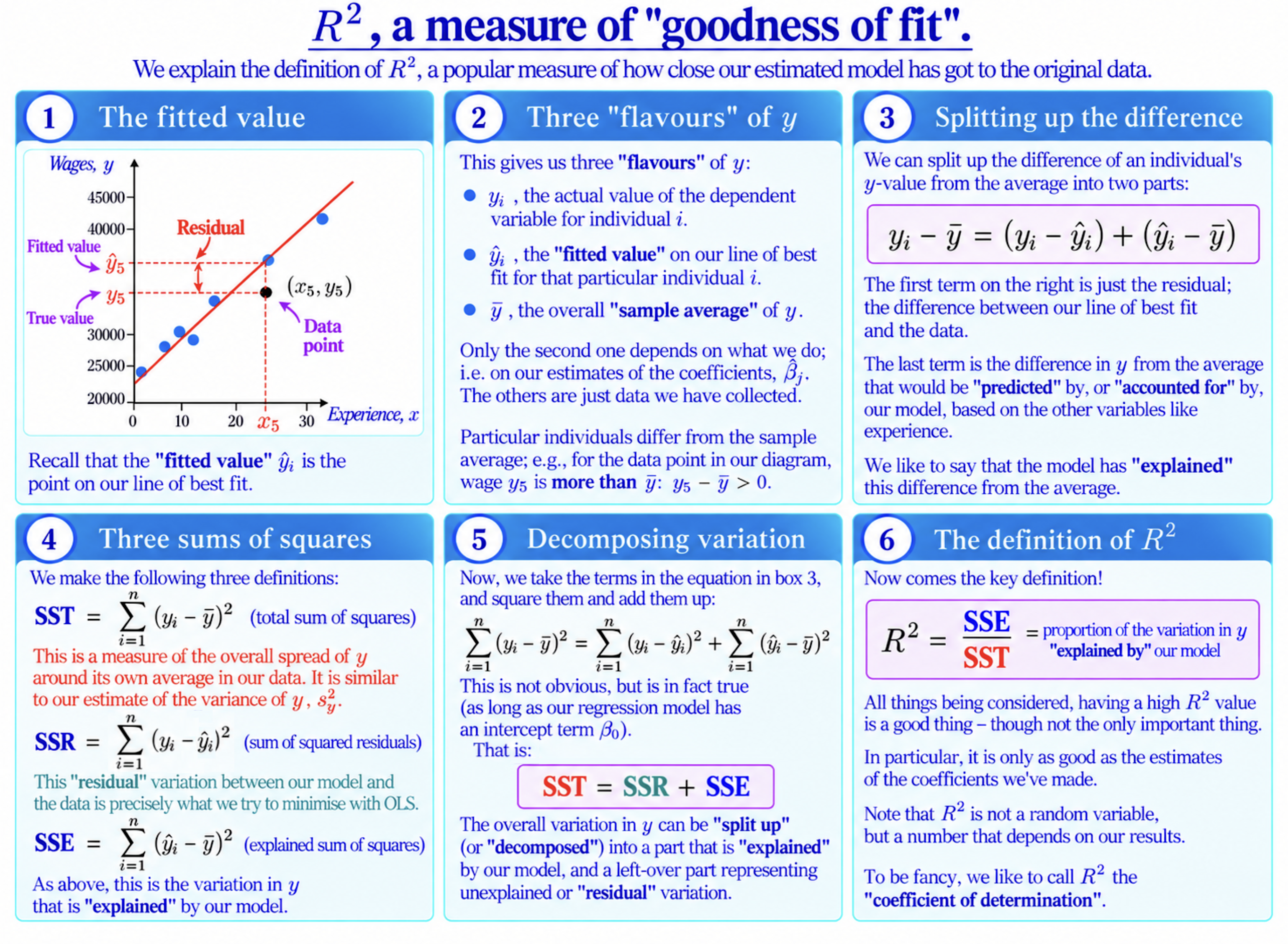
$R^2$ and Model Fit

Once we have estimated a regression model, a natural question is:

How closely does our fitted model match the data?

In a simple linear regression model, this is just asking how close our “line of best fit” has managed to get to the data.

Perhaps the most common way to summarise this is using $R^2$, usually read as “R-squared”.

To be clear about its definition, we first need to recap three different but related concepts to do with the dependent variable $Y$.

Three “Flavours” of $y$

Once we have collected our sample, for each individual $i$, we have three things:

• $y_i$: the actual value of the dependent variable in the data for individual $i$
• $\hat{y}_i$: the fitted value, as predicted by our estimated model, for individual $i$
• $\bar{y}$: the overall sample average of all the $y_i$ we have collected

For example, in our wage and experience model, $y_i$ is somebody’s actual wage, while $\hat{y}_i$ is the wage represented by the point on our fitted regression line at that person’s level of experience, and $\bar{y}$ is the average wage of the workers we asked.

Note also that only one of the three depends on the model we have estimated: $\hat{y}_i$. The actual value $y_i$ and the sample average $\bar{y}$ come directly from the data, and can’t be changed by anything we do.

Splitting Up the Difference from the Average

An individual’s observed value $y_i$ may be above or below the overall sample average $\bar{y}$. This difference from the average invites explanation.

We begin by taking this difference:

$$y_i-\bar{y}$$

and rewriting it by splitting it into two parts:

$$y_i-\bar{y}=(y_i-\hat{y}_i)+(\hat{y}_i-\bar{y})$$

Note that the $\hat{y}_i$ terms cancel.

Now, the second term,

$$\hat{y}_i-\bar{y}$$

is our model’s prediction of how far this individual should be from the sample average.

For example, suppose somebody earns more than the average worker in our sample. Based only on their experience and our fitted regression line, we might also predict them to earn more than average. The amount by which their fitted wage $\hat{y}_i$ differs from the average wage $\bar{y}$ is the difference from the average that our model predicts them to have.

So, we might say that this is the part of their deviation from the average that is “predicted by”, or “accounted for” by the model. Actually, we especially like to use the term “explained by” the model – though we usually stop short of using causal language.

Meanwhile, the first term,

$$y_i-\hat{y}_i$$

we should recognise as the residual. It measures the part of the individual’s deviation that our fitted model has not accounted for. For a simple linear regression, it is precisely the vertical difference of the data point from the OLS line, as shown in the diagram.

Recall also that it was the sum of squares of these residuals that we tried to minimise with OLS in the first place.

Three Sums of Squares

We now square these three deviations and add them across all $n$ observations.

First, the total sum of squares is

$$SST=\sum_{i=1}^{n}(y_i-\bar{y})^2$$

This measures the total variation of the observed $y_i$ around their sample average.

Next, the sum of squared residuals is

$$SSR=\sum_{i=1}^{n}(y_i-\hat{y}_i)^2$$

This measures the residual variation left between the fitted model and the observed data.

Recall that this is exactly the quantity that OLS chooses our fitted line to minimise.

Finally, the explained sum of squares is

$$SSE=\sum_{i=1}^{n}(\hat{y}_i-\bar{y})^2$$

This measures the variation in $y$ that is accounted for by the fitted values from our model.

A word of warning here: unfortunately, there is also an alternative convention in use. Some people use these terms in exactly the opposite way, writing “SSR” for “regression sum of squares” (meaning our SSE), and “SSE” or “sum of squared errors” for our SSR, even though these are not errors but residuals.

We don’t take kindly to these types around here. If you see anyone using this notation, remember to stare at them rudely.

Decomposing the Variation

As long as our OLS regression has an intercept, these three quantities satisfy:

$$SST=SSR+SSE$$

So, the total variation in $y$ can be decomposed into two parts:

$$\text{total variation}=\text{residual variation}+\text{explained variation}$$

This is the key relationship behind the definition of $R^2$.

The Definition of $R^2$

Now comes the most important bit! We define:

$$R^2=\frac{SSE}{SST}$$

So, $R^2$ is the proportion of the total variation in $y$ that is accounted for by our fitted model.

Using

$$SST=SSR+SSE$$

we can equivalently write

$$R^2=1-\frac{SSR}{SST}$$

So, since SST is fixed, the smaller the SSR is, the larger $R^2$ will be.

Interpreting $R^2$

A larger $R^2$ means that the fitted values lie closer, overall, to the observed data relative to the total variation in $y$.

So, all else being equal, a higher $R^2$ indicates a closer fit to the sample data.

But this is only a statement about model fit. A high $R^2$ does not by itself tell us that our estimated coefficients have the interpretation we want, or that the model is good in every other respect.

We will return to these interpretive questions later.

Finally, notice that $R^2$ is calculated after we have observed the data and estimated the regression. It is therefore a number describing our fitted model, rather than a random variable.

Another name for $R^2$ is the coefficient of determination.

Background

• Residuals vs Errors
• Lines of Best Fit
• OLS Estimation